Introduction to Artificial Intelligence - Homework Assignment 01 (5 pts.)

• Names:
• NETIDs:

This assignment covers the following topics:

• Cleaning and splitting a mixed pandas dataset
• Feature engineering from text and numerical evidence
• Implementing k-Nearest Neighbors and validating it against scikit-learn
• Feature engineering from categorical activity data
• Training and interpreting a Decision Tree classifier

It consists of six tasks:

Task ID	Description	Points
00	Load and split the polygraph dataset	0.5
01	Engineer features from polygraph evidence	1
02	Implement, validate, and tune a kNN classifier	1.5
03	Collect, load, and combine structured suspect statements	0.5
04	Engineer activity features and train a Decision Tree	1.5
05	Export the completed notebook	0
	Total	5

Please complete all sections. Some questions require written answers, while others involve coding. Run your code cells in order to verify your solutions.

Story Progression

Late one evening, the police received an emergency call from the William Theisen-Floyd Estate, where an elaborate dinner party has ended in murder. By the time the authorities arrived, the host, William Theisen-Floyd, had been found dead in the pantry. The scene suggests that he was killed with gas, but the guests disappeared before they could be questioned.

Evidence 1: The grisly scene discovered in the estate's pantry.

The police know that six guests attended the party — three men and three women — but every name on the guest list appears to be an alias:

• Colonel Mustard
• Professor Plum
• Mr. Green
• Miss Scarlet
• Mrs. Peacock
• Mrs. White

Evidence 2: A photograph of William Theisen-Floyd with the six unidentified guests shortly before his murder.

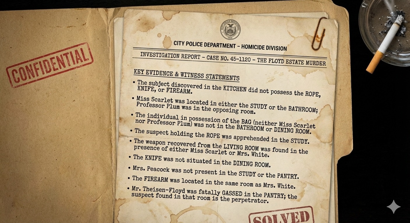
Investigators searched the estate's bathroom, dining room, kitchen, living room, pantry, and study. In those rooms they recovered six possible weapons: a bag, a firearm, gas, a knife, poison, and a rope. Witness accounts and clues left around the estate allowed the police to reconstruct the party.

• Colonel Mustard had been in the dining room with the poison
• Professor Plum in the bathroom with the knife
• Miss Scarlet in the study with the rope
• Mrs. Peacock in the kitchen with the bag
• Mrs. White in the living room with the firearm.

Most importantly, Mr. Green had been in the pantry with the gas. The police now know which alias belongs to the murderer — but an alias is not a person they can arrest.

Evidence 3: The police report containing the clues recovered while searching the estate.

Evidence 4: A witness places Mr. Green near the pantry on the night of the murder.

A few days later, as you finish your drink, you feel a tap on your shoulder.

"You've got the wrong person, pal."

When you turn around, you find Officer Gaff waiting behind you. He assures you that you are not under arrest — at least not today — and drives you to the precinct to meet Director Bryant. The department has followed every conventional lead it has, but it still cannot connect the six aliases to the guests' real identities. Director Bryant has heard that you know something about artificial intelligence, or at least that you are currently enrolled in a class with those words in its title, and decides that this is close enough for police work.

The police have assembled a broad pool of possible suspects and asked each one ten questions about the night of the murder while administering a polygraph examination. For every response, they recorded both the suspect's statement and the estimated probability that the suspect was lying. They also have sixty labeled examples from earlier investigations that describe how likely a person with particular polygraph results was to merit further investigation. Unfortunately, the department's intern handed the data processing to Gemini, and the historical examples and current suspect interviews have all been mixed together in a single file named suspect_data.csv.

Evidence 5: One of the possible suspects undergoing a police polygraph examination.

Director Bryant slides the evidence file across the desk. Before the aliases can be unmasked, you will need to separate the historical training records from the current interviews, transform the suspects' raw answers into features a machine-learning algorithm can understand, and implement a classifier capable of narrowing the field. Somewhere in that list is the person who called themself Mr. Green.

Task 00: Load and Split Dataset

Task 00-1: Description (0 pts.)

Loading the Dataset

Run the cell below to download the evidence, load suspect_data.csv into a DataFrame, and display its first five rows.

Task 00-1: Code (0 pts.)

import os
import shutil
import subprocess
from pathlib import Path

REPO_URL = 'https://github.com/wtheisen/nd-cse-30124-homeworks.git'

try:
    import google.colab
except ImportError:
    # Reuse a local checkout, including when launched from a homework subfolder.
    DATA_ROOT = next((p for p in [Path.cwd(), *Path.cwd().parents]
                      if (p / '.git').exists() and (p / 'evidence').is_dir()), None)
    if DATA_ROOT is None:
        DATA_ROOT = Path.cwd() / 'nd-cse-30124-homeworks'
else:
    # Leave the old checkout before deleting it, including on a setup-cell rerun.
    os.chdir('/content')
    DATA_ROOT = Path('/content/nd-cse-30124-homeworks')
    # Fetch fresh evidence every time this cell runs in Colab.
    if DATA_ROOT.exists():
        shutil.rmtree(DATA_ROOT)

if not DATA_ROOT.exists():
    subprocess.run(['git', 'clone', REPO_URL, str(DATA_ROOT)], check=True)

if not (DATA_ROOT / '.git').exists():
    raise RuntimeError(f'{DATA_ROOT} exists but is not a Git checkout. Choose a different clone location.')

# All later relative paths now start at the homework repository root.
os.chdir(DATA_ROOT)
DATA_ROOT = Path.cwd()

import pandas as pd

# TODO
# Load suspect_data.csv into a pandas DataFrame.
suspect_df = None

suspect_df.head()

Task 00-1: Reference Output (0 pts.)

suspect_name	weapon_mentions	total_lying_prob	good_suspect	statement_1	statement_2	statement_3	statement_4	statement_5	statement_6	...	lying_prob_1	lying_prob_2	lying_prob_3	lying_prob_4	lying_prob_5	lying_prob_6	lying_prob_7	lying_prob_8	lying_prob_9	lying_prob_10
0	Clair Green	NaN	NaN	NaN	I arrived late to the party	Someone was carrying a bag upstairs	I heard arguing in the study	The buffet in the kitchen looked incomplete	I stayed near the entrance	Someone mentioned a knife was missing	...	0.50	0.52	0.49	0.51	0.50	0.52	0.49	0.51	0.50	0.51
1	Amelie Boom	3.0	0.77	1.0	NaN	NaN	NaN	NaN	NaN	NaN	...	NaN	NaN	NaN	NaN	NaN	NaN	NaN	NaN	NaN	NaN
2	Kaila Bryant	4.0	0.85	1.0	NaN	NaN	NaN	NaN	NaN	NaN	...	NaN	NaN	NaN	NaN	NaN	NaN	NaN	NaN	NaN	NaN
3	Amelie Boom	NaN	NaN	NaN	I arrived alone	I mingled with guests	The host mentioned a knife collection	I stayed in common areas	I left at midnight	Nothing caught my eye	...	0.54	0.53	0.55	0.54	0.53	0.55	0.54	0.53	0.54	0.55
4	Dannylo Correia	3.0	0.86	1.0	NaN	NaN	NaN	NaN	NaN	NaN	...	NaN	NaN	NaN	NaN	NaN	NaN	NaN	NaN	NaN	NaN

Note: Colab will format this DataFrame as a scrollable table.

Task 00-2: Description (0 pts.)

Splitting the Dataset

Separate the combined DataFrame into two new DataFrames using pandas: one containing the 60 labeled examples from prior cases, where good_suspect is either 0 or 1, and one containing the interviews from the 20 suspects in the current case, where good_suspect is NaN. The examples below introduce the pandas operations needed for this task.

Checking for Missing Values

# Count NaN values in each column
df.isna().sum()

# Check if a specific column has NaN values
df['column_name'].isna()  # Returns True/False for each row

# Filter to rows where a column is NOT NaN
df[df['column_name'].notna()]

Inspecting Data Types

df.info()  # Shows data type and non-null count for each column
df.dtypes  # Just shows data types

Filtering DataFrames with Conditional Indexing

# Basic filtering
adults = df[df['age'] >= 18]           # Rows where age is 18+
students = df[df['role'] == 'student'] # Rows where role is 'student'

# Filtering by NaN values
has_email = df[df['email'].notna()]    # Rows where email is NOT NaN
no_email = df[df['email'].isna()]      # Rows where email IS NaN

# Multiple conditions (use & for AND, | for OR)
young_students = df[(df['age'] < 25) & (df['role'] == 'student')]

Important: When using multiple conditions, wrap each condition in parentheses.

Task 00-2: Code (0.5 pts.)

# TODO
# Split rows with known labels into training_df and rows with missing labels into testing_df.
training_df = None
testing_df = None

print(f"Training samples: {len(training_df)}")
print(f"Testing samples: {len(testing_df)}")
print(f"Total: {len(training_df) + len(testing_df)}")

Task 00-2: Reference Output (0 pts.)

Training samples: 60
Testing samples: 20
Total: 80

Story Progression

You can't believe the police mixed the training and testing data together in one file — Professor Theisen would have killed you for that. I guess that's what happens when an intern blindly delegates the data processing to AI. Fortunately, you separated the records and can now see that:

• Training data: (60 records) has weapon_mentions, total_lying_prob, and good_suspect (the label).
• Testing data: (20 records) has raw statement_1 through statement_10 and lying_prob_1 through lying_prob_10.

Unfortunately, the testing data format doesn't match the training data format. You'll need to do some feature engineering to transform the raw testing data into the same format as the training data!

Feature engineering is the process of transforming raw data into meaningful numerical values ("features") that machine-learning algorithms can use. Good features can make a simple algorithm work well, while poor features can make even a sophisticated algorithm fail.

We'll need to create two features from the raw polygraph data in order to match our examples:

1. weapon_mentions (count feature): How many times weapon-related keywords appear in the suspect's statements
2. total_lying_prob (aggregate feature): The average lying probability across all statements

Task 01: Create Features from Testing Data to Match Training Data

Task 01-1: Description (0 pts.)

Creating the Weapon Mention Feature

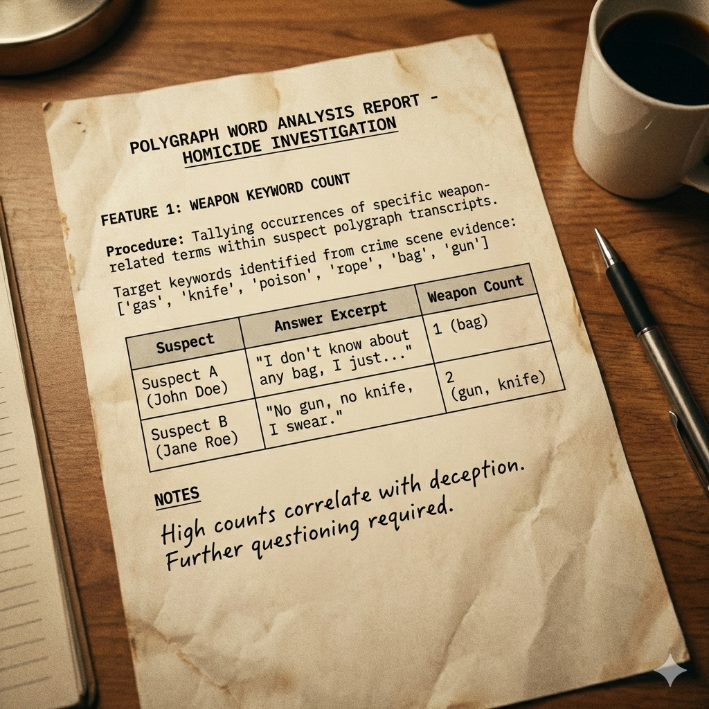
Our first feature counts how many times weapon-related keywords appear in a suspect's polygraph answers. Use the following canonical list:

weapons = ['gas', 'knife', 'poison', 'rope', 'bag', 'gun']

These terms correspond to the possible weapons identified by police at the crime scene.

Evidence 6: Mapping polygraph answers to weapon mentions.

Useful String Operations in Pandas

# Convert to lowercase (important for matching!)
text = "I saw a KNIFE"
text.lower()  # Returns: "i saw a knife"

# Count occurrences of a substring
text = "the knife was a sharp knife"
text.count('knife')  # Returns: 2

# Join multiple strings together
statements = ["I was home", "I saw nothing", "I left early"]
combined = ' '.join(statements)  # "I was home I saw nothing I left early"

Using df.apply() to Process Each Row

When you need to apply a custom function to each row of a DataFrame, use df.apply() with axis=1:

def my_function(row):
    # row is a pandas Series representing one row
    # You can access columns like: row['column_name']
    return some_value

# Apply to each row and create a new column
df['new_column'] = df.apply(my_function, axis=1)

# Or use a lambda (anonymous function) for simple operations
df['new_column'] = df.apply(lambda row: row['a'] + row['b'], axis=1)

Requirements

Complete count_weapon_mentions() so that it:

1. Combines the ten statement columns for one suspect.
2. Converts the combined text to lowercase.
3. Counts every occurrence of the six weapon keywords.
4. Returns the total count for that suspect.

Documentation

• DataFrame.apply()
• str.lower()
• str.count()

Task 01-1: Code (0.5 pts.)

weapons = ['gas', 'knife', 'poison', 'rope', 'bag', 'gun']

def count_weapon_mentions(row, weapons):
    """
    Count how many weapon keywords appear across all statements for a suspect.

    Args:
        row (pandas.Series): A pandas Series representing one suspect's data
        weapons (list): List of weapon keywords to search for

    Returns:
        weapon_count (int): Total count of weapon mentions
    """
    # TODO
    # Select the ten statement columns, combine and lowercase their text, then count every weapon-keyword occurrence.
    statement_columns = None
    combined_statements = None

    return sum(combined_statements.count(weapon) for weapon in weapons)

testing_df['weapon_mentions'] = testing_df.apply(
    lambda row: count_weapon_mentions(row, weapons), axis=1
)

print("Weapon mentions per suspect:")
print(testing_df[['suspect_name', 'weapon_mentions']].head(10))

Task 01-1: Reference Output (0 pts.)

Weapon mentions per suspect:
           suspect_name  weapon_mentions
0           Clair Green                2
3           Amelie Boom                1
9          Kaila Bryant                1
14      Dannylo Correia                0
16     Stephen Playford                0
18     Grace Sparwasser                0
22      William Theisen                6
26  Alexander Nwanganga                6
32      Annika Svensson                0
37     Maureen Tremblay                1

Task 01-2: Description (0 pts.)

Creating the Average Lying Probability Feature

The second missing feature is total_lying_prob. If several polygraph answers have a high estimated probability of deception, the suspect should appear more suspicious overall. We want one number that summarizes that pattern.

Aggregation Methods

There are several ways to combine multiple values into one:

Method	Function	When to use
Mean (average)	np.mean()	When all values contribute equally
Sum	np.sum()	When you want total amount
Max	np.max()	When the highest value matters most
Min	np.min()	When the lowest value matters most
Median	np.median()	When you want to ignore outliers

Example Calculation

import numpy as np

# A suspect's lying probabilities for 10 statements
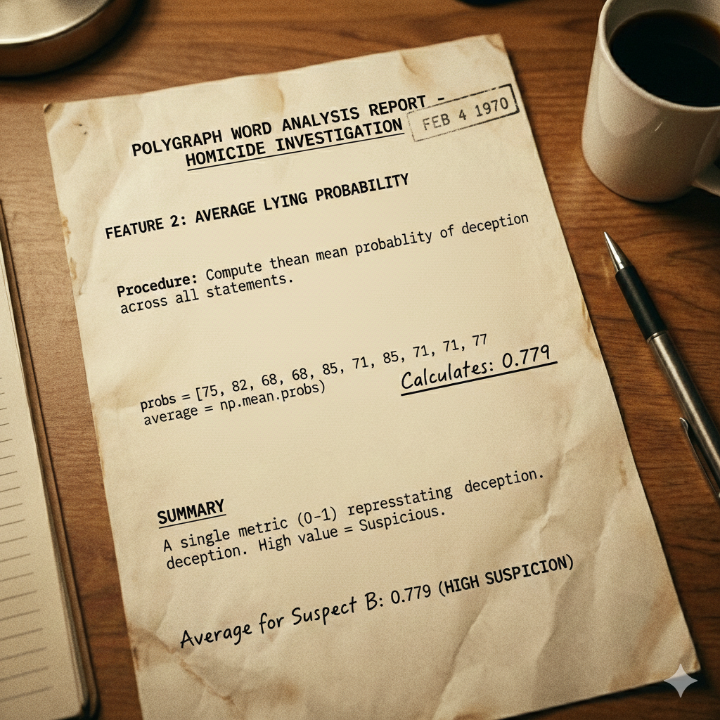
probs = [0.75, 0.82, 0.68, 0.79, 0.85, 0.71, 0.88, 0.73, 0.81, 0.77]

# Calculate average
average = np.mean(probs)  # Returns: 0.779

We will use the mean (average) of all lying probabilities. This produces a single value between 0 and 1 representing the average estimated probability of deception.

Requirements

Complete avg_lying_probs() so that it:

1. Retrieves the ten lying-probability values for one suspect.
2. Computes their arithmetic mean.
3. Returns the resulting value.

Evidence 7: Averaging polygraph lying probabilities.

Documentation

• numpy.mean()

Task 01-2: Code (0.5 pts.)

import numpy as np

def avg_lying_probs(row):
    """
    Extract all lying probability values from a row and calculate their average.

    Args:
        row (pandas.Series): A pandas Series representing one suspect's data

    Returns:
        avg (float): Average lying probability (between 0 and 1)
    """
    # TODO
    # Select every lying_prob_* column and return its mean.
    lying_probability_columns = None

    return np.mean(row[lying_probability_columns].astype(float))

# TODO
# Apply avg_lying_probs() to every testing row.
testing_df['total_lying_prob'] = None

print("Total lying probability (average) per suspect:")
print(testing_df[['suspect_name', 'total_lying_prob']].head(10))

Task 01-2: Reference Output (0 pts.)

Total lying probability (average) per suspect:
           suspect_name  total_lying_prob
0           Clair Green             0.505
3           Amelie Boom             0.540
9          Kaila Bryant             0.540
14      Dannylo Correia             0.175
16     Stephen Playford             0.175
18     Grace Sparwasser             0.175
22      William Theisen             0.784
26  Alexander Nwanganga             0.783
32      Annika Svensson             0.177
37     Maureen Tremblay             0.537

Task 01-3: Description (0 pts.)

Preparing Feature Matrices for Machine Learning

Now that we've created our features, we need to convert the data into the format that our classification models can use.

Scikit-learn's Data Format

Scikit-learn algorithms expect data in a consistent format:

Variable	Shape	Description	Example
X	(n_samples, n_features)	Feature matrix	[[4, 0.85], [0, 0.12], [3, 0.78]]
y	(n_samples,)	Target labels	[1, 0, 1]

• X is a 2D array where each row is one sample (suspect) and each column is one feature
• y is a 1D array of labels (what we're trying to predict)

Converting DataFrame to NumPy Array

# Select specific columns and convert them to a NumPy array
X = df[['feature1', 'feature2']].to_numpy()

# Get labels
y = df['label_column'].to_numpy()

Requirements

Create X_train, y_train, and X_test using the two engineered features in the same column order.

Documentation

• DataFrame.to_numpy()

Task 01-3: Code (0 pts.)

feature_columns = ['weapon_mentions', 'total_lying_prob']

# TODO
# Build the training feature matrix, training-label vector, and testing feature matrix using the same ordered feature columns.
X_train = None
y_train = None
X_test = None

Task 01-3: Reference Output (0 pts.)

Note: No printed output is expected from this setup cell.*

Task 02: Implement kNN to Find the Suspects

Unlike many machine-learning algorithms, k-Nearest Neighbors does not construct a model during training. It stores the labeled examples and performs the following steps for every new example:

1. Calculate the distance from the new example to every training example.
2. Select the k training examples with the smallest distances.
3. Collect those neighbors' labels.
4. Predict the label that occurs most often.

You will implement these steps yourself. Do not use scikit-learn's KNeighborsClassifier until Task 02-3, where it will serve as a reference implementation for checking your work.

Task 02-1: Description (0 pts.)

Distance and Neighbor Selection

For two feature vectors (\mathbf{x}) and (\mathbf{z}), Euclidean distance is:

[ d(\mathbf{x}, \mathbf{z}) = \sqrt{\sum_i (x_i-z_i)^2} ]

Complete euclidean_distance() and find_k_nearest_neighbors() below. The latter should calculate one distance per training example, then return the indices of the k smallest distances. np.argsort() may be useful: it returns the indices that would arrange an array from smallest to largest.

Coding Reference

NumPy performs arithmetic on arrays element by element:

import numpy as np

point_a = np.array([2.0, 0.50])
point_b = np.array([5.0, 0.80])

differences = point_a - point_b       # array([-3.0, -0.3])
squared = differences ** 2            # array([9.0, 0.09])
total = np.sum(squared)                # 9.09
distance = np.sqrt(total)              # approximately 3.015

np.argsort() returns indices rather than sorted values. This is useful because the indices let us retrieve the corresponding labels afterward:

distances = np.array([0.8, 0.2, 1.1, 0.4])
sorted_indices = np.argsort(distances) # array([1, 3, 0, 2])
nearest_two = sorted_indices[:2]       # array([1, 3])

Argument	Purpose
point_a, point_b	Two one-dimensional feature vectors of equal length
X_train	A two-dimensional array with one labeled training example per row
query_point	The new feature vector whose neighbors we want to find
k	The number of nearest training examples to return

Documentation

• numpy.sum()
• numpy.sqrt()
• numpy.argsort()

Task 02-1: Code (0.5 pts.)

def euclidean_distance(point_a, point_b):
    """Return the Euclidean distance between two one-dimensional arrays."""
    # TODO
    # Implement Euclidean distance using NumPy operations.
    differences = None
    squared_differences = None

    return np.sqrt(np.sum(squared_differences))


def find_k_nearest_neighbors(X_train, query_point, k):
    """Return the row indices of the k training examples nearest query_point."""
    # TODO
    # Calculate all distances and return the indices of the k smallest values.
    distances = None

    return np.argsort(distances)[:k]


example_distance = euclidean_distance(X_train[0], X_test[0])
example_neighbors = find_k_nearest_neighbors(X_train, X_test[0], k=3)

print(f"Distance from the first training example to the first suspect: {example_distance:.4f}")
print(f"Indices of the three nearest neighbors: {example_neighbors.tolist()}")
print(f"Labels of the three nearest neighbors: {y_train[example_neighbors].tolist()}")

Task 02-1: Reference Output (0 pts.)

Distance from the first training example to the first suspect: 1.0345
Indices of the three nearest neighbors: [38, 12, 17]
Labels of the three nearest neighbors: [0.0, 0.0, 1.0]

Task 02-2: Description (0 pts.)

Majority Vote and Batch Prediction

Now use the neighbor indices to make a prediction. predict_one_knn() should:

1. Find the nearest neighbors.
2. Retrieve their labels from y_train.
3. Count the votes for each class.
4. Return the class with the most votes.

You may use np.bincount() to count integer labels and np.argmax() to find the label with the largest count. Then complete predict_knn() so it calls your single-example function once for every row in X_test.

We use odd values of k in this assignment, so the two classes cannot tie.

Coding Reference

Suppose the nearest-neighbor indices and the complete training labels are:

neighbor_indices = np.array([4, 1, 7])
y_train_example = np.array([0, 1, 0, 1, 1, 0, 0, 1])

neighbor_labels = y_train_example[neighbor_indices]
# array([1, 1, 1])

vote_counts = np.bincount(neighbor_labels, minlength=2)
# array([0, 3]): zero votes for class 0 and three votes for class 1

prediction = np.argmax(vote_counts)
# 1

The minlength=2 argument guarantees one vote counter for each of our two classes, even when no neighbor votes for one of them. np.argmax() returns the index of the largest count, and that index is also our class label.

To generate predictions for several query points, use the same single-example function repeatedly:

predictions = []
for query_point in X_test:
    prediction = some_prediction_function(query_point)
    predictions.append(prediction)

predictions = np.array(predictions)

Argument	Purpose
X_train	Training feature matrix
y_train	Known class label for each training row
query_point	One current suspect's feature vector
X_test	All current suspects' feature vectors
k	Number of neighbors participating in the vote

Documentation

• numpy.bincount()
• numpy.argmax()

Task 02-2: Code (0.5 pts.)

def predict_one_knn(X_train, y_train, query_point, k):
    """Predict the class of one query point using majority vote."""
    # Retrieve neighbor labels, count their votes, and return the majority class.
    neighbor_indices = None
    neighbor_labels = None

    vote_counts = None

    return int(np.argmax(vote_counts))


def predict_knn(X_train, y_train, X_test, k):
    """Predict one class label for every row in X_test."""
    # TODO
    # Call predict_one_knn() for every test row and return a NumPy array of predictions.
    predictions = None

    return np.array(predictions)


student_predictions = predict_knn(X_train, y_train, X_test, k=3)
testing_df['knn_prediction'] = student_predictions.astype(float)
knn_suspects = testing_df[testing_df['knn_prediction'] == 1]

print(f"kNN (k=3) identified {len(knn_suspects)} suspects to investigate further:")
print(knn_suspects[['suspect_name', 'weapon_mentions', 'total_lying_prob', 'knn_prediction']].to_string())

Task 02-2: Reference Output (0 pts.)

kNN (k=3) identified 6 suspects to investigate further:
           suspect_name  weapon_mentions  total_lying_prob  knn_prediction
3           Amelie Boom                1             0.540             1.0
9          Kaila Bryant                1             0.540             1.0
22      William Theisen                6             0.784             1.0
26  Alexander Nwanganga                6             0.783             1.0
37     Maureen Tremblay                1             0.537             1.0
76           Kaiwen Shi                4             0.779             1.0

Story Progression

Hmm—that's odd. Several of these suspects have alibis for the night of the murder; you know, for example, that Amelie was supporting the cheer squad at a basketball game that evening. Something must have gone wrong. You wonder whether a different value of k might affect the results. It may be worth trying several hyperparameters. A hyperparameter is a value you choose before training that affects how the model behaves. Unlike model parameters, which are learned from data, hyperparameters are selected by you.

Task 02-3: Description (0 pts.)

Hyperparameter Selection

Hyperparameter Examples

Algorithm	Hyperparameter	What it controls
kNN	n_neighbors (k)	How many neighbors to consider
Decision Tree	max_depth	How deep the tree can grow
Neural Network	learning_rate	How fast to update weights

Effect of k in kNN

• Small k (e.g., 1 or 3):

  • More sensitive to local patterns
  • Can be influenced by noise/outliers
  • May overfit

• Large k (e.g., 10 or 20):

  • More robust to noise
  • Smoother decision boundaries
  • May underfit (miss local patterns)

Requirements

Before relying on a new algorithm implementation, it is important to compare it against a trusted reference. For each value in [1, 3, 5, 7, 9]:

1. Generate predictions with your predict_knn() function.
2. Fit a scikit-learn KNeighborsClassifier with the same value of k.
3. Generate its predictions and check whether the two arrays are identical.
4. Print the suspects selected by your implementation.

Coding Reference

Scikit-learn classifiers use a consistent three-step interface:

from sklearn.neighbors import KNeighborsClassifier

reference_model = KNeighborsClassifier(n_neighbors=3)
reference_model.fit(X_train, y_train)
reference_predictions = reference_model.predict(X_test)

Call or Argument	Purpose
n_neighbors=k	Use the same number of neighbors as your implementation
.fit(X_train, y_train)	Store the labeled training examples
.predict(X_test)	Return one predicted label for each test row
np.array_equal(a, b)	Return True only when two arrays have identical values and shape

The reference model must receive the same feature arrays and value of k as your implementation; otherwise the comparison would not test equivalent algorithms.

Documentation

• KNeighborsClassifier
• numpy.array_equal()

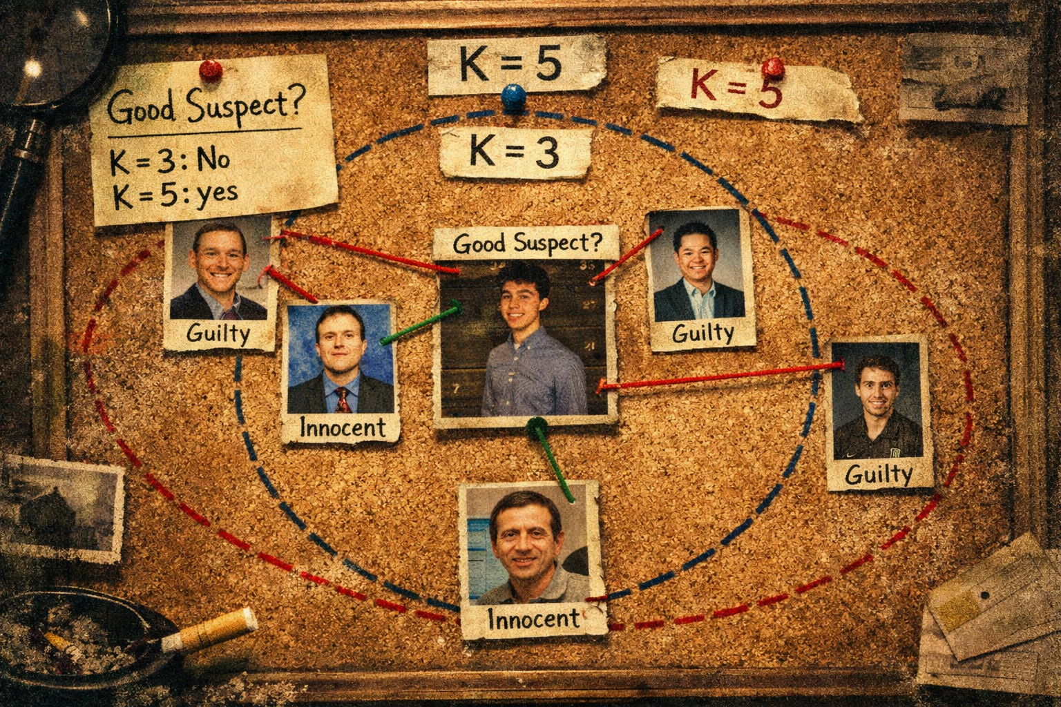
Important: Every comparison should print True. If one does not, debug your implementation before continuing. The final three values of k should produce:

['Clair Green', 'William Theisen', 'Alexander Nwanganga', 'Quinn Hynes', 'Arda Kurama', 'Kaiwen Shi']

Evidence 8: Implementing and validating kNN.

Task 02-3: Code (0.5 pts.)

from sklearn.neighbors import KNeighborsClassifier

for k in [1, 3, 5, 7, 9]:
    # TODO
    # Generate predictions from the handwritten implementation.
    student_predictions = None

    # TODO
    # Configure, fit, and query the equivalent sklearn model.
    reference_model = None
    reference_predictions = None

    predictions_match = np.array_equal(student_predictions, reference_predictions)

    testing_df['knn_prediction'] = student_predictions.astype(float)
    knn_suspects = testing_df[testing_df['knn_prediction'] == 1]

    print(
        f"k={k}: matches sklearn = {predictions_match} | "
        f"{len(knn_suspects)} suspects - {knn_suspects['suspect_name'].tolist()}"
    )

Task 02-3: Reference Output (0 pts.)

k=1: matches sklearn = True | 6 suspects - ['Amelie Boom', 'Kaila Bryant', 'William Theisen', 'Alexander Nwanganga', 'Maureen Tremblay', 'Kaiwen Shi']
k=3: matches sklearn = True | 6 suspects - ['Amelie Boom', 'Kaila Bryant', 'William Theisen', 'Alexander Nwanganga', 'Maureen Tremblay', 'Kaiwen Shi']
k=5: matches sklearn = True | 6 suspects - ['Clair Green', 'William Theisen', 'Alexander Nwanganga', 'Quinn Hynes', 'Arda Kurama', 'Kaiwen Shi']
k=7: matches sklearn = True | 6 suspects - ['Clair Green', 'William Theisen', 'Alexander Nwanganga', 'Quinn Hynes', 'Arda Kurama', 'Kaiwen Shi']
k=9: matches sklearn = True | 6 suspects - ['Clair Green', 'William Theisen', 'Alexander Nwanganga', 'Quinn Hynes', 'Arda Kurama', 'Kaiwen Shi']

Story Progression

The selected suspects change with k, which is a useful warning against trusting a single hyperparameter choice. You leave the changing names for the police to investigate cautiously, but three people appear in every result:

• Kaiwen Shi
• Alexander Nwanganga
• William Theisen

These three must be especially suspicious. It may be worth paying one of them a visit on your own time...

The kNN model identifies the strongest leads, but that evidence alone is not enough to charge anyone. Investigators next compare each suspect's account of the evening with historical activity patterns associated with the six aliases.

For k=5, k=7, and k=9, your implementation settles on the same six-person shortlist — the same number as the six unidentified guests at the estate. That stable result is a useful lead, but a polygraph score and a few weapon-related words cannot tell the police which suspect used which alias, much less prove who committed the murder.

Evidence 9: A blueprint of the estate and the rooms described in the suspects' statements.

Director Bryant has another source of evidence. The estate's historical records describe where each alias tended to spend time and what kinds of activities were associated with them during the evening of the party. The police have matching statements from most of the six suspects, but one record was never digitized: William Theisen still has the only paper copy of his statement. Collect that final sheet, preserve it with the exported evidence, and compare all six suspects' activity patterns against the known aliases.

Task 03: Collect, Load, and Combine Structured Statements

Task 03-1: Description (0 pts.)

The kNN results provide a shortlist, but the polygraph features do not explain what the suspects were doing during the evening. The police have provided historical alias activity samples and complete statements for five of the six suspects. One statement sheet is still missing.

Before completing this task, obtain the single statement sheet from Professor William Theisen during his office hours. You will convert its 20 observations into a small DataFrame and add it to the provided evidence.

Requirements

Use the CSV evidence files in evidence/homework01/:

1. Load alias_statements.csv into alias_df (2400 rows).
2. Load suspect_statements.csv into suspect_statements_df (100 rows representing five suspects).
3. Encode William Theisen's collected sheet as a 20-row DataFrame with the columns suspect_name, statement_index, time, location, and activity. The starter code includes the first two observations as examples; extend that list with the remaining 18 observations from the sheet.
4. Concatenate the collected statements with the provided statements to produce 120 rows representing all six suspects.
5. Define the canonical suspect, alias, room, and weapon lists used by the feature-engineering code.

Coding Reference

When DataFrames have the same columns and should be stacked vertically, use pd.concat():

combined_df = pd.concat([df_a, df_b], ignore_index=True)

ignore_index=True creates a clean row index after the records are combined.

Documentation

• pandas.concat()

Check: When the collected sheet has been entered correctly, the cell reports 2,400 alias rows, 100 provided suspect rows, 20 collected William rows, and 120 combined suspect rows.

Task 03-1: Code (0.5 pts.)

import pandas as pd

alias_df = pd.read_csv(DATA_ROOT / "evidence/homework01/alias_statements.csv")
suspect_statements_df = pd.read_csv(
    DATA_ROOT / "evidence/homework01/suspect_statements.csv"
)

# TODO
# Transcribe the 20 observations from William's collected sheet
# into a DataFrame with the required five columns.
william_rows = pd.DataFrame([
    {"suspect_name": "William Theisen", "statement_index": i,
     "time": time, "location": location, "activity": activity}
    for i, (time, location, activity) in enumerate([
        ("19:00 PM", "Study", "Opening letters"),
        ("19:10 PM", "Study", "Reading a novel quietly"),
    ])
])

suspect_statements_df = pd.concat(
    [suspect_statements_df, william_rows], ignore_index=True
)

ALIASES = ['Colonel Mustard', 'Miss Scarlet', 'Mr. Green',
           'Mrs. Peacock', 'Mrs. White', 'Professor Plum']
ROOMS = ['Study', 'Dining Room', 'Kitchen', 'Pantry', 'Living Room', 'Bathroom']
WEAPONS = ['Poison', 'Knife', 'Gas', 'Rope', 'Bag', 'Firearm']
SUSPECTS = [
    'Clair Green', 'William Theisen', 'Alexander Nwanganga',
    'Quinn Hynes', 'Arda Kurama', 'Kaiwen Shi'
]

# Keep the downstream decision-tree output in the same order as the kNN shortlist.
suspect_statements_df = pd.concat(
    [
        suspect_statements_df[suspect_statements_df['suspect_name'] == suspect]
        for suspect in SUSPECTS
    ],
    ignore_index=True,
)

print(f"Alias statement rows: {len(alias_df)}")
print(f"Provided suspect statement rows: {len(suspect_statements_df) - len(william_rows)}")
print(f"Collected William statement rows: {len(william_rows)}")
print(f"Combined suspect statement rows: {len(suspect_statements_df)}")
print(f"Suspects: {SUSPECTS}")

Task 03-1: Reference Output (0 pts.)

Alias statement rows: 2400
Provided suspect statement rows: 100
Collected William statement rows: 20
Combined suspect statement rows: 120
Suspects: ['Clair Green', 'William Theisen', 'Alexander Nwanganga', 'Quinn Hynes', 'Arda Kurama', 'Kaiwen Shi']

Story Progression

Looking through the new evidence, you notice many repeated locations and overlapping activities. These are categorical data. You wonder whether a decision tree could treat the six aliases as classes and match each suspect's statement pattern against them.

Task 04: Decision Trees

Task 04-1: Description (0 pts.)

Feature Engineering

First, we need to convert the categorical evidence into numerical features. Two useful feature groups are the proportion of time a person spends in each room and whether their activities suggest any of the possible weapons.

Evidence 10: Converting categorical features to numerical ones.

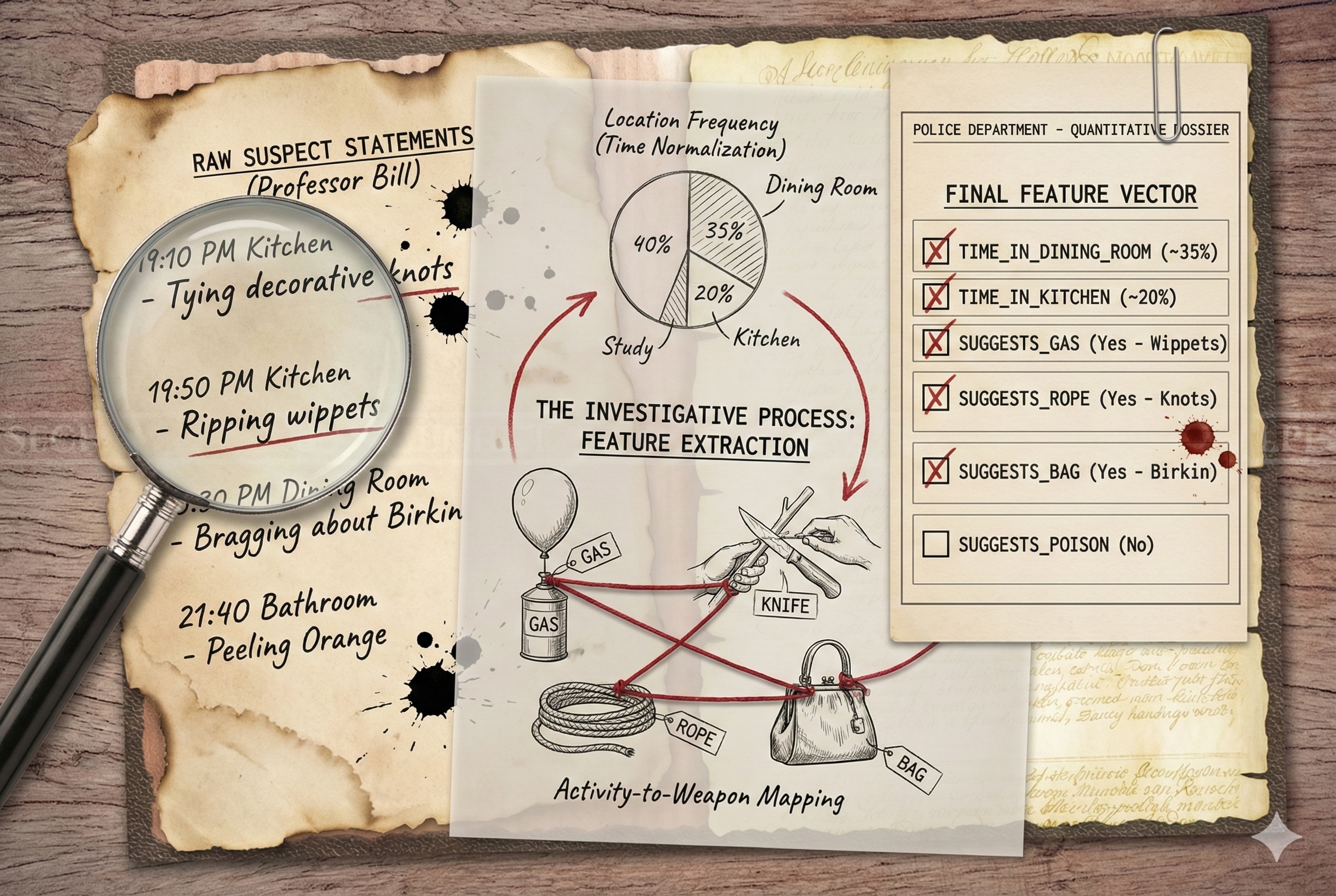
Requirements

Complete extract_features() so that it returns the room-proportion and weapon-activity features defined in the starter code.

Coding Reference: Counting Categorical Values

When you have a column of categorical data and want to count how many times each value appears, use value_counts():

locations = df['location']
location_counts = locations.value_counts()
# Returns a Series like:
#   Study          8
#   Kitchen        5
#   Dining Room    3
#   ...

# Access a specific count (returns 0 if the value isn't found)
location_counts.get('Study', 0)  # Returns: 8
location_counts.get('Pantry', 0)  # Returns: 0

Coding Reference: Mapping Categorical Values

When you want to convert every value in a column using a dictionary lookup, use Series.map():

weapon_map = {'Opening a safe': 'Firearm', 'Taking her dog for a walk': 'Rope'}

# Map each activity to its weapon (unmapped activities become NaN)
weapons_used = df['activity'].map(weapon_map)
# Returns a Series like:
#   0    Firearm
#   1        NaN    <- activity wasn't in the dictionary
#   2       Rope

# Use .dropna() to remove NaN values
weapons_used.dropna()  # Only keeps the successfully mapped values

Note: .map() is cleaner than writing a loop containing repeated dictionary-membership checks.

Documentation

• Series.value_counts()
• Series.map()

Task 04-1: Code (0.5 pts.)

# Each weapon is represented by three associated activities.
activity_weapon_mapping = {
    'Inflating balloons': 'Gas',
    'Ripping wippets': 'Gas',
    # TODO: Supply the third Gas activity.

    'Whittling a stick': 'Knife',
    'Peeling an orange': 'Knife',
    'Opening letters': 'Knife',

    'Tampering with drinks': 'Poison',
    'Rinsing a glass carefully': 'Poison',
    # TODO: Supply the third Poison activity.

    'Tying decorative knots': 'Rope',
    'Raising a painting': 'Rope',
    'Taking her dog for a walk': 'Rope',

    'Inspecting a family heirloom': 'Firearm',
    'Opening a safe': 'Firearm',
    'Talking about skeet shooting': 'Firearm',

    'Bragging about their Birkin': 'Bag',
    'Complaining about TSA going through their purse': 'Bag',
    # TODO: Supply the third Bag activity.
}

def extract_features(statements_df: pd.DataFrame) -> dict:
    """Convert categorical room and activity observations to numeric features."""
    rooms = ['Study', 'Dining Room', 'Kitchen', 'Pantry', 'Living Room', 'Bathroom']
    weapons = ['Poison', 'Knife', 'Gas', 'Rope', 'Bag', 'Firearm']

    features = {}
    total_time = len(statements_df)

    # TODO
    # Count room visits and convert them to proportions.
    location_counts = None
    for room in rooms:
        features[f'time_in_{room}'] = None

    # TODO
    # Student prompt: Map activities to weapons and create one binary feature per weapon.
    suggested_weapons = set(
        None
    )

    for weapon in weapons:
        features[f'suggests_{weapon}'] = None

    return features

Task 04-1: Reference Output (0 pts.)

Note: No printed output is expected when the feature-engineering function is defined.*

Task 04-2: Description (0 pts.)

Preparing Data for Classification

Now that extract_features() produces numerical values, we can prepare the historical alias data for training and the suspect data for classification.

Requirements

Create the following two DataFrames:

• alias_features_df: one row per alias sample, with columns for alias_name, alias_sample_id, plus all feature columns
• suspect_features_df: one row per suspect, with columns for suspect_name plus all feature columns

Coding Reference

Earlier in this notebook, we used df.apply(func, axis=1) to run a function on each row. Here, we need to run a function on each group of rows. Each alias has 20 sample statements, and we want to extract features from each sample separately.

groupby() splits a DataFrame into groups based on one or more columns, then apply() runs a function on each group:

# Group by alias_name and sample_id, then extract features from each group
alias_features_df = alias_df.groupby(['alias_name', 'alias_sample_id']) \
    .apply(lambda g: pd.Series(extract_features(g)), include_groups=False) \
    .reset_index()

The chained operations have the following roles:

Step	What it does
.groupby(['alias_name', 'alias_sample_id'])	Splits the DataFrame into one sub-DataFrame per unique (alias, sample) pair
.apply(lambda g: ...)	Calls the lambda on each sub-DataFrame g
extract_features(g)	Calls the Task 04-1 function, which returns a dictionary of features
pd.Series(...)	Converts the dict into a pandas Series (one row of data)
include_groups=False	Don't pass the grouping columns into the function
.reset_index()	Converts the group keys back into regular columns

Documentation

• DataFrame.groupby()
• GroupBy.apply()

Task 04-2: Code (0 pts.)

import pandas as pd
from sklearn.tree import DecisionTreeClassifier
from sklearn.tree import export_text

alias_features_df = alias_df.groupby(['alias_name', 'alias_sample_id'], sort=False) \
    .apply(lambda g: pd.Series(extract_features(g)), include_groups=False).reset_index()

suspect_features_df = suspect_statements_df.groupby('suspect_name', sort=False) \
    .apply(lambda g: pd.Series(extract_features(g)), include_groups=False).reset_index()

Task 04-2: Reference Output (0 pts.)

Note: No printed output is expected when the feature DataFrames are constructed.*

Task 04-3: Description (0 pts.)

Decision Tree Classifier

Now that both datasets use the same numerical feature columns, we can train a decision tree on the historical aliases and apply it to the six suspects.

Unlike kNN, you will use scikit-learn for the tree construction. The objective is to learn the library's model interface and connect its arguments to the tree concepts discussed in lecture.

Requirements

Scikit-learn expects a two-dimensional feature matrix and a one-dimensional label array:

Variable	Contents	Shape in this task
X_alias	Numerical features for historical alias samples	(120, 12)
y_alias	Alias label for each historical sample	(120,)
X_suspects	Numerical features for the six suspects	(6, 12)

Select columns from a DataFrame and convert them to NumPy like this:

feature_columns = ['feature_a', 'feature_b']
X = dataframe[feature_columns].to_numpy(dtype=float)
y = dataframe['label'].to_numpy()

Coding Reference

from sklearn.tree import DecisionTreeClassifier

model = DecisionTreeClassifier(
    criterion='entropy',
    random_state=42,
    max_depth=4,
    min_samples_split=4,
)
model.fit(X_train, y_train)
probabilities = model.predict_proba(X_test)

Argument or Attribute	Purpose
criterion='entropy'	Evaluate candidate splits using entropy and information gain
random_state=42	Make any randomized choices reproducible
max_depth=4	Prevent the tree from growing beyond four levels
min_samples_split=4	Require at least four examples before splitting a node
.fit(X, y)	Construct the tree from labeled examples
.predict_proba(X)	Return one probability per possible alias for every test row
.classes_	Alias labels in the same column order as predict_proba()

For example, if model.classes_[2] is 'Mr. Green', then column 2 of the probability matrix contains every suspect's estimated probability of matching Mr. Green.

Documentation

• DecisionTreeClassifier
• DecisionTreeClassifier.predict_proba()

Task 04-3: Code (0 pts.)

# Define feature columns (same rooms and weapons from extract_features)
feature_cols = [f'time_in_{room}' for room in ROOMS] + [f'suggests_{weapon}' for weapon in WEAPONS]

# TODO
# Construct the decision-tree training matrix and label vector.
X_alias = None
y_alias = None

# TODO
# Configure the specified entropy-based tree and fit it to the historical alias data.
clf = None

clf.fit(X_alias, y_alias)

# TODO
# Construct the suspect feature matrix and obtain class probabilities from the fitted tree.
X_suspects = None
probabilities = None

print("\nProbability of Each Suspect Matching Each Alias:\n")
print(f"{clf.classes_}")

aliases = list(clf.classes_)

for suspect_name, probs in zip(suspect_features_df['suspect_name'], probabilities):
    formatted_probs = [f"{value:.4f}" for value in probs]
    print(f'{suspect_name}: {formatted_probs}')

dt_results_df = pd.DataFrame(
    probabilities,
    index=suspect_features_df['suspect_name'].values,
    columns=aliases,
)

Task 04-3: Reference Output (0 pts.)

Probability of Each Suspect Matching Each Alias:

['Colonel Mustard' 'Miss Scarlet' 'Mr. Green' 'Mrs. Peacock' 'Mrs. White' 'Professor Plum']
Clair Green: ['0.0000', '0.0000', '0.0000', '1.0000', '0.0000', '0.0000']
William Theisen: ['0.0000', '0.0000', '0.0000', '0.0000', '0.0000', '1.0000']
Alexander Nwanganga: ['0.5000', '0.0000', '0.0000', '0.5000', '0.0000', '0.0000']
Quinn Hynes: ['0.0000', '0.0000', '0.8636', '0.0000', '0.0455', '0.0909']
Arda Kurama: ['0.0000', '0.9412', '0.0000', '0.0000', '0.0000', '0.0588']
Kaiwen Shi: ['0.0000', '0.2000', '0.0000', '0.0000', '0.8000', '0.0000']

Task 04-4: Description (0 pts.)

Decision Tree Short Answer Questions

Answer both questions in the written-response section below.

Task 04-4: Written Response (0.5 pts.)

1. Why are we using criterion='entropy'? Explain what "entropy" means in this context and what the tree is maximizing at each split.

   Answer: [ANSWER]

2. Do we need to scale or normalize our features for a decision tree? Why or why not?

   Answer: [ANSWER]

Story Progression

The activity evidence gives you a leading match: the Decision Tree assigns Quinn Hynes to Mr. Green with substantially greater confidence than any other alias. Combined with the earlier deduction that Mr. Green was in the pantry with the gas, Quinn is now the investigation's leading suspect.

You call Detective Caulfield and explain what the models found. He is less impressed than you hoped. A polygraph-based nearest-neighbor classification and a decision-tree probability may justify further investigation, but they are not enough to charge anyone or obtain a warrant on their own. You submit the new report with Quinn's name at the top and begin looking for a more direct piece of evidence that can turn a statistical lead into a case.

Task 05: Export the Completed Notebook

Task 05-1: Description (0 pts.)

Export the Completed Notebook

Set GENERATE = True in the following cell and run it after completing the assignment. Colab will export the notebook as an HTML file for submission.

Important: Run all earlier cells in order before exporting so that your submitted HTML includes your answers and outputs.

Task 05-1: Code (0 pts.)

import json
import os
import subprocess

ASS_PATH = "nd-cse-30124-homeworks/homeworks"
ASS = "homework01"
GENERATE = False

if GENERATE:
    try:
        from google.colab import _message, files

        repo_ipynb_path = f"/content/{ASS_PATH}/{ASS}/{ASS}.ipynb"
        nb = _message.blocking_request("get_ipynb", timeout_sec=1)["ipynb"]

        os.makedirs(os.path.dirname(repo_ipynb_path), exist_ok=True)
        with open(repo_ipynb_path, "w", encoding="utf-8") as f:
            json.dump(nb, f)

        !jupyter nbconvert --to html "{repo_ipynb_path}"
        files.download(repo_ipynb_path.replace(".ipynb", ".html"))
    except Exception:
        nb_fp = os.path.join(os.getcwd(), f"{ASS}.ipynb")
        subprocess.run(["jupyter", "nbconvert", "--to", "html", nb_fp], check=True)

Task 05-1: Reference Output (0 pts.)

When GENERATE = True, Colab converts the completed notebook to HTML and begins downloading homework01.html.