Introduction to Artificial Intelligence - Homework Assignment 02 (5 pts.)
- Name:
- NETID:
This assignment covers the following topics:
- Writing a linear model and finding its weights with ordinary least squares
- Fitting polynomial models with four different degrees
- Writing Ridge regression and choosing a model using validation data
- Applying the chosen model to held-out records from the mansion
| Task ID | Description | Points |
|---|---|---|
| 00 | Load the historical records | 0.25 |
| 01 | Write prediction and loss functions | 0.5 |
| 02 | Find the straight-line weights with OLS | 1 |
| 03 | Check against scikit-learn | 0.25 |
| 04 | Write and compare four polynomial models | 0.75 |
| 05 | Write Ridge regression and choose the best model | 1.25 |
| 06 | Evaluate on the held-out mansion set and explain the result | 1 |
| 07 | Export the completed notebook | 0 |
| Total | 5 |
Please complete all sections, including written answers, and run cells in order.
Story Progression
Thanks to your work in HW01, Quinn Hynes is the leading match for Mr. Green. He was seen inflating balloons in the kitchen and pantry and mentioned that canisters were stored there. Caulfield would like something a little more convincing than “our classifier said so,” so let's follow up on the balloons.
The police found records of the party preparations, including the balloons filled and the weight of a gas canister before and afterward. The canister got lighter, as you would expect. But did it lose more gas than the balloons should have used?
Apparently our next contribution to the murder investigation is a model of party supplies. We'll learn from earlier filling jobs, check how well we can predict new ones, and then see what the mansion's records tell us.

Task 00: Prepare Historical Evidence
Task 00-1: Description (0 pts.)
Loading the Party Records
The police have collected records from earlier balloon-filling jobs. Each row tells us the volume of balloons filled and how much lighter the gas canister was afterward. We'll use those examples to predict how much gas the mansion's party preparations should have used.
We need two columns:
balloon_volume_liters: the volume of the filled balloons in liters. This is our input.mass_loss_g: the canister's weight loss in grams. This is what we're predicting.
trial_id just identifies the job; leave it out of the model. The data loading is done for you below, much like HW01.
We'll use three sets of records:
- Historical (Train): earlier jobs used to find each model's weights.
- Validation (Val): separate experiments used to compare models and choose a winner.
- Mansion (Test): records from the party preparations, saved until our model is chosen.
The files are historical.csv, case_validation.csv, and mansion.csv. All three download together, but leave the mansion file closed until Task 06. We want to choose our model before seeing the answers we're investigating!
Python Help
df = pd.read_csv('historical.csv')
print(df.head())
Useful Links
Task 00-1: Code (0 pts.)
import os
import shutil
import subprocess
from pathlib import Path

REPO_URL = 'https://github.com/wtheisen/nd-cse-30124-homeworks.git'

try:
    import google.colab
except ImportError:
    # Reuse a local checkout, including when launched from a homework subfolder.
    DATA_ROOT = next((p for p in [Path.cwd(), *Path.cwd().parents]
                      if (p / '.git').exists() and (p / 'evidence').is_dir()), None)
    if DATA_ROOT is None:
        DATA_ROOT = Path.cwd() / 'nd-cse-30124-homeworks'
else:
    # Leave the old checkout before deleting it, including on a setup-cell rerun.
    os.chdir('/content')
    DATA_ROOT = Path('/content/nd-cse-30124-homeworks')
    # Fetch fresh evidence every time this cell runs in Colab.
    if DATA_ROOT.exists():
        shutil.rmtree(DATA_ROOT)

if not DATA_ROOT.exists():
    subprocess.run(['git', 'clone', REPO_URL, str(DATA_ROOT)], check=True)

if not (DATA_ROOT / '.git').exists():
    raise RuntimeError(f'{DATA_ROOT} exists but is not a Git checkout. Choose a different clone location.')

# All later relative paths now start at the homework repository root.
os.chdir(DATA_ROOT)
DATA_ROOT = Path.cwd()

EVIDENCE_DIR = DATA_ROOT / 'evidence' / 'homework02'

if not (EVIDENCE_DIR / 'mansion.csv').exists():
    raise FileNotFoundError(
        f'HW02 evidence is missing from {DATA_ROOT}. Rerun setup in Colab after the corrected evidence is published; locally, update this checkout with git pull --ff-only.'
    )

# Enter the evidence folder so the remaining cells can use simple filenames.
os.chdir(EVIDENCE_DIR)

import numpy as np
import pandas as pd

historical_df = pd.read_csv('historical.csv')
quinn_statements = pd.read_csv('hw01_quinn_statements.csv')

FEATURE_COLUMN, TARGET_COLUMN = 'balloon_volume_liters', 'mass_loss_g'
TARGET_UNIT = 'grams'
FEATURE_LOW, FEATURE_HIGH = 20., 96.

def extract_feature(df):
    return df[FEATURE_COLUMN].to_numpy(dtype=float)

print(historical_df.head().to_string(index=False))
print(f'Historical jobs: {len(historical_df)}')
Task 00-1: Expected Output (0 pts.)
trial_id  balloon_volume_liters  mass_loss_g
     H01                   20.0     3.114080
     H02                   24.0     4.028029
     H03                   28.0     4.494672
     H04                   32.0     6.266059
     H05                   36.0     4.536902
Historical jobs: 12
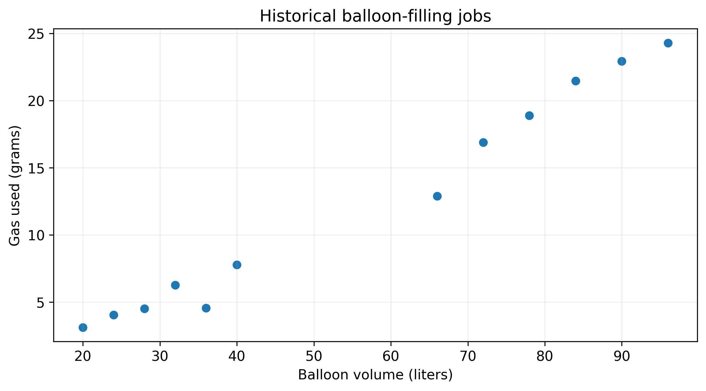
Note: The plot below is not part of the expected output, it's just here to help you visualize the data.
Task 00-2: Description (0 pts.)
Choosing Our Input and Output
First, put the balloon volumes in x_train and the measured weight losses in y_train. Use FEATURE_COLUMN for the input and TARGET_COLUMN for the target, converting both to a NumPy array. Both should have shape (12,), one number per job.
Keep the rows in the same order so each volume still goes with the correct weight. Then look at the supplied output: there's quite a gap between some of our measurements. Keep that in mind when we start drawing curves through them.

Python Help
y = df['target'].to_numpy(dtype=float)
Useful Links
Task 00-2: Code (0.25 pts.)
#TODO: Load the feature and target columns and convert to numpy floats
x_train = None
y_train = None

print(f'Feature shape: {x_train.shape}; target shape: {y_train.shape}')
print(f'Feature range: {x_train.min():.4f} to {x_train.max():.4f}')
Task 00-2: Expected Output (0 pts.)
Feature shape: (12,); target shape: (12,)
Feature range: 20.0000 to 96.0000
Task 01: Implement Prediction and Loss
Task 01-1: Description (0 pts.)
Turning the Data into Predictions
In class, we wrote our predictions as $\hat{y}=Xw$. Let's turn that into code. Each row of $X$ describes one job, and each entry in $w$ tells us how much a feature contributes to the prediction.
For our first model, a row looks like $[1,x]$ and the weights are $[w_0,w_1]$. Multiplying them gives $w_0+w_1x$: the familiar equation for a line. The column of ones lets us include the intercept in the same multiplication as the slope.
Complete create_input by adding that column of ones. Then complete predict_linear using matrix multiplication. In NumPy, @ does matrix multiplication; * multiplies matching entries instead.
Our input matrix will have shape (12, 2), the weights will have shape (2,), and the predictions will have shape (12,). Later we'll give the model more columns, but these same two functions will still work.
Python Help
features = np.array([[2.], [4.]])
ones = np.ones(features.shape[0])
X_example = np.column_stack((ones, features))
# [[1., 2.], [1., 4.]]
# @ performs matrix multiplication; * multiplies element by element.
Useful Links
Task 01-1: Code (0 pts.)
def create_input(features):
    features = np.asarray(features, dtype=float)

    # TODO: Add a column of 1s to our matrix to represent the y-intercept
    return None

def predict_linear(X, weights):
    # TODO: Perform a matrix multiplication to create our predictions
    return None

example = predict_linear(create_input(np.array([2., 4.])), np.array([1., 3.]))

print(f'Example predictions: {example}')
Task 01-1: Expected Output (0 pts.)
Example predictions: [ 7. 13.]
Task 01-2: Description (0 pts.)
How Wrong Are Our Predictions?
Before we can decide which line fits best, we need a way to measure its mistakes. Subtract each prediction from the measured value to get a residual. If a canister lost 10 grams and we predicted 8, the residual is 2 grams: we predicted too little.
We'll square each residual and take the average. This is mean squared error, or MSE:
$$ \mathrm{MSE}=\frac{1}{n}\sum_{i=1}^{n}(y_i-\hat{y}_i)^2. $$
Squaring keeps positive and negative mistakes from canceling each other out. Be careful to square the individual errors before averaging them!
Complete mean_squared_error and check the examples below. We'll often report its square root, RMSE, because that puts the error back in grams and makes it easier to interpret.
Python Help
errors = np.array([1., -2., 2.])
print(np.mean(errors**2))  # 3.0
Useful Links
Task 01-2: Code (0.5 pts.)
def mean_squared_error(y_true, y_pred):
    # TODO: Calculate MSE
    residuals = None

    return None
Task 02: Fit the Historical Straight-Line Baseline
Task 02-1: Description (0 pts.)
Finding the Best Weights with OLS
Now we can make predictions and measure their errors. How do we find the weights that make those errors as small as possible?
This is the OLS calculation we worked through in class. The equation looks a bit imposing, but we've already written most of the surrounding pieces. Starting with the sum of squared errors, we set the gradient to zero:
$$ L(w)=\|Xw-y\|_2^2,\qquad 2X^{\top}(Xw-y)=0. $$
Rearranging gives
$$ X^{\top}Xw=X^{\top}y,\qquad \hat{w}=(X^{\top}X)^{-1}X^{\top}y. $$
Complete fit_ols by calculating the transpose, the two matrix products, and the weights. We'll use np.linalg.solve for the last step. It solves the same equation without making us explicitly calculate the inverse. The small example below shows how to use it.
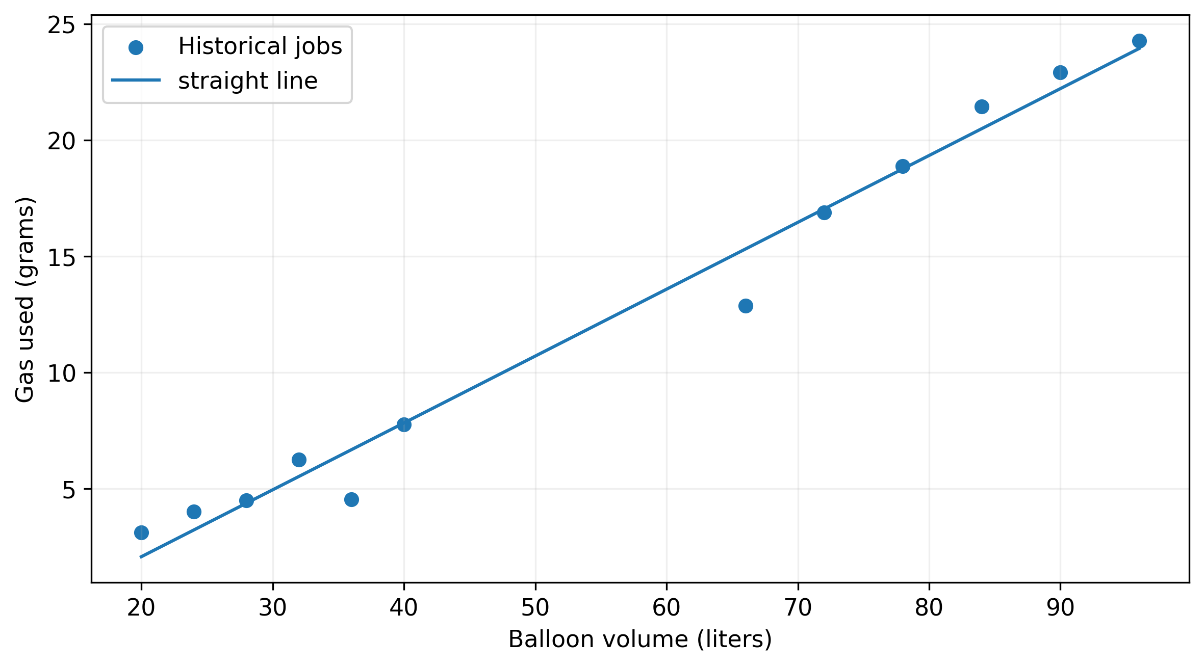
The returned array should contain the intercept first and the slope second. Use your prediction function to see how the fitted line does on the historical jobs. The figure below shows the line and the mistakes it still makes. Is there a pattern in those mistakes?
Two details to keep in mind: minimizing MSE gives the same OLS weights as minimizing SSE, since we only divided by the number of examples. Also, not every matrix has an inverse; the supplied check catches cases where the columns cannot give us a unique answer. We'll return to the numerical issue when we fit a much more flexible curve.
Python Help
A = np.array([[2., 0.], [0., 4.]])
c = np.array([6., 8.])
z = np.linalg.solve(A, c)  # [3., 2.], satisfying A @ z == c
transpose = A.T
Useful Links
Task 02-1: Code (1 pts.)
def fit_ols(X, y):
    # TODO: Calculate the weights via OLS

    return weights

# TODO: generate predictions for X_train with the fit model
X_train = None
linear_weights = None
train_predictions = None

line_train_rmse = np.sqrt(mean_squared_error(y_train, train_predictions))

print(f'Input shape: {X_train.shape}; weight shape: {linear_weights.shape}')
print(f'Intercept w0: {linear_weights[0]:.6f}; slope w1: {linear_weights[1]:.6f}')
print(f'Straight-line historical RMSE: {line_train_rmse:.4f} grams')
Task 02-1: Expected Output (0 pts.)
Design shape: (12, 2); weight shape: (2,)
Intercept w0: -3.677931; slope w1: 0.287778
Straight-line historical RMSE: 1.0941 grams
Note: This plot below isn't part of your expected output, it's just here to help you visualize what we're doing.
Task 03: Verify the Implementation
Task 03-1: Description (0 pts.)
Does Scikit-learn Agree with Us?
Let's see how our handmade regression compares to scikit-learn! Fit LinearRegression on the same historical jobs and check its weights, predictions, and MSE against yours. They should match apart from tiny rounding differences.
Remember that scikit-learn supplies its own intercept, so don't give it our column of ones. Use x_train.reshape(-1, 1) as its input. Its coef_[0] is the slope and intercept_ is the intercept; the supplied checks take care of rounding. Get all four checks passing before moving on.
Python Help
from sklearn.linear_model import LinearRegression
reference = LinearRegression().fit(x_train.reshape(-1, 1), y_train)
predictions = reference.predict(x_train.reshape(-1, 1))
Useful Links
Task 03-1: Code (0.25 pts.)
from sklearn.linear_model import LinearRegression
from sklearn.metrics import mean_squared_error as sklearn_mse

# TODO: Use scikit learn to produce predictions on the same data
reference_model = None
reference_predictions = None

checks = {
    'Slope': np.isclose(linear_weights[1], reference_model.coef_[0]),
    'Intercept': np.isclose(linear_weights[0], reference_model.intercept_),
    'Predictions': np.allclose(train_predictions, reference_predictions),
    'MSE': np.isclose(mean_squared_error(y_train, train_predictions), sklearn_mse(y_train, reference_predictions)),
}

for label, value in checks.items(): print(f'{label} matches: {bool(value)}')
Task 03-1: Expected Output (0 pts.)
Slope matches: True
Intercept matches: True
Predictions matches: True
MSE matches: True
Story Progression
Our line agrees with scikit-learn! Now let's see whether a curve can do a better job. We will try four degrees on the same historical records, then compare their predictions on the validation jobs.

Task 04: Write and Compare Polynomial Models
Task 04-1: Description (0 pts.)
Giving Our Model a Curve
A straight line uses $1$ and $x$. A quadratic adds $x^2$, so its prediction is $w_0+w_1x+w_2x^2$. We can keep adding powers to make more flexible curves. We still find a weight for each column and add the results, just as we did for the line.
Complete polynomial_features so that degree 3 produces columns $u$, $u^2$, and $u^3$. Leave out the ones column; our create_input function adds it later. Then complete fit_polynomial to find the weights using np.linalg.lstsq(X, y, rcond=None)[0].
This is still ordinary least squares. We use lstsq here because high powers can make the earlier normal-equation calculation unreliable. It finds the weights directly without forming $X^{\top}X$.
The supplied preparation code rescales the input and puts the power columns on comparable scales. You don't need to write that part. It learns its scale from the historical jobs and reuses it for every later prediction.
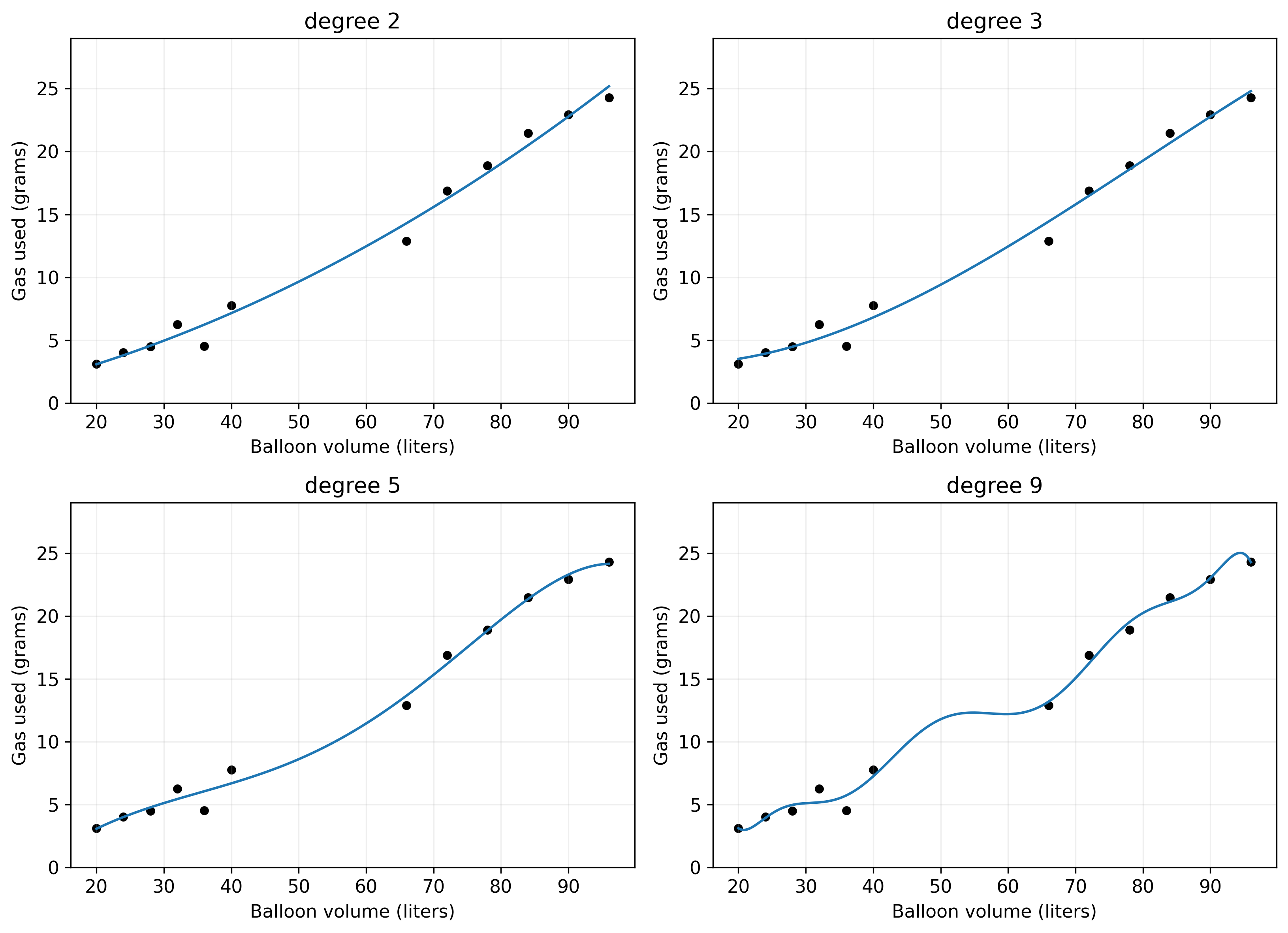
We'll compare degrees 2, 3, 5, and 9. The last one has ten weights, including the intercept, for only twelve historical jobs. That is a lot of freedom!
Python Help
powers = [u**power for power in range(1, degree + 1)]
columns = np.column_stack(powers)
Task 04-1: Code (0.5 pts.)
from sklearn.preprocessing import StandardScaler

def polynomial_features(u, degree):
    # TODO: Compute the polynomial features to add to our input matrix
    return None

def fit_polynomial(X, y):
    # TODO: Compute the weights using np.linalg.lstsq()
    return None

# GIVEN: scale each feature once using historical data only.
def domain_coordinate(x):
    return 2 * (np.asarray(x) - FEATURE_LOW) / (FEATURE_HIGH - FEATURE_LOW) - 1

degrees = [2, 3, 5, 9]
scalers, training_matrices = {}, {}
for degree in degrees:
    raw = polynomial_features(domain_coordinate(x_train), degree)
    scaler = StandardScaler().fit(raw)
    scalers[degree] = scaler
    training_matrices[degree] = design_matrix(scaler.transform(raw))

def matrix_for(x, degree):
    raw = polynomial_features(domain_coordinate(x), degree)
    return create_input(scalers[degree].transform(raw))

def rmse(y_true, predictions):
    return np.sqrt(mean_squared_error(y_true, predictions))

# A single collection will hold the line, curves, and later Ridge models.
candidates = [{'name': 'straight line', 'degree': 1, 'alpha': 0.,
               'weights': linear_weights}]

for degree in degrees:
    # TODO: find the weights for each degree
    weights = None

    candidates.append({'name': f'degree {degree}', 'degree': degree,
                       'alpha': 0., 'weights': weights})

def predict_candidate(candidate, x):
    X = create_input(x) if candidate['degree']==1 else matrix_for(x, candidate['degree'])

    return predict_linear(X, candidate['weights'])

for candidate in candidates:
    error = rmse(y_train, predict_candidate(candidate, x_train))

    print(f"{candidate['name']}: historical RMSE = {error:.4f} grams")
Task 04-1: Expected Output (0 pts.)
straight line: historical RMSE = 1.0941 grams
degree 2: historical RMSE = 0.8472 grams
degree 3: historical RMSE = 0.8075 grams
degree 5: historical RMSE = 0.6787 grams
degree 9: historical RMSE = 0.5890 grams
NOTE: The plots below aren't part of your expected output, but they ARE the actual curves you're fitting
Task 04-2: Description (0 pts.)
Which Curves Predict New Jobs?
The police ran another batch of balloon-filling experiments. These are our validation jobs: we know the answers, but none of the models used them to find its weights.
Complete the two error calculations below. The resulting table compares the line and all four curves on historical and validation jobs. Lower RMSE means better predictions.
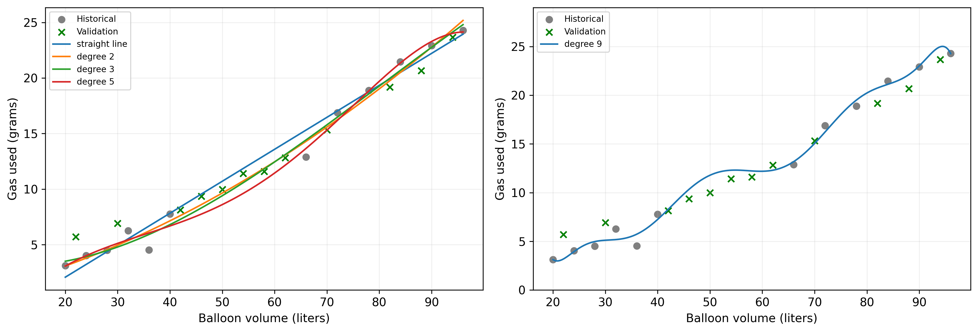
Look for a model that fits the old jobs closely but struggles on the new jobs. That is overfitting. We will keep all five candidates in the comparison while we try Ridge next. We have not chosen our final model yet.
Python Help
error = rmse(actual, predictions)
Task 04-2: Code (0.25 pts.)
validation_df = pd.read_csv('case_validation.csv')

# TODO: Read in the val data and convert to numpy float
x_validation = None
y_validation = None

def compare_candidates(candidates):
    rows = []
    for candidate in candidates:
        # TODO: Calculate the rmse for the train and the val datasets
        historical_error = None
        validation_error = None

        rows.append({'model': candidate['name'], 'degree': candidate['degree'],
                     'alpha': candidate['alpha'], 'historical_rmse': historical_error,
                     'validation_rmse': validation_error})

    return pd.DataFrame(rows)

plain_comparison = compare_candidates(candidates)
print(plain_comparison.to_string(index=False, float_format=lambda v: f'{v:.4f}'))
Task 04-2: Reference Output (0 pts.)
model  degree  alpha  historical_rmse  validation_rmse
straight line       1 0.0000           1.0941           1.3153
     degree 2       2 0.0000           0.8472           1.0508
     degree 3       3 0.0000           0.8075           1.1031
     degree 5       5 0.0000           0.6787           1.4186
     degree 9       9 0.0000           0.5890           1.3416
NOTE: The plot below is not part of your expected output but is a nice visualization of the above comparison
Story Progression
The intern points out that the degree-nine curve fits the old records beautifully. Caulfield points to its predictions on new jobs. We need a way to stop a flexible model from chasing every bump in the old measurements.

Task 05: Write Ridge Regression and Choose a Model
Task 05-1: Description (0 pts.)
Adding a Cost for Large Weights
Caufield is worried about possible overfitting, something simple regressions can be prone to. One solution to prevent overfitting is to try and use a regularization like L1 (LASSO) or L2 (RIDGE).
Ridge keeps the same polynomial columns, but changes how we choose their weights. Along with the prediction error, we add a cost for large weights:
$$ L(w)=\|Xw-y\|_2^2+\alpha\sum_{j=1}^{d}w_j^2. $$
The sum starts at $j=1$ because we leave the intercept $w_0$ alone. A larger alpha puts more pressure on the feature weights to stay small. The model may fit the historical points less closely, but it can make better predictions on new jobs.
Here we use the sum of squared errors, so alpha has the same meaning as in scikit-learn. We will still use RMSE to compare predictions.
Like OLS, Ridge gives us an equation for the weights:
$$ (X^{\top}X+\alpha P)w=X^{\top}y. $$
$P$ is an identity matrix with its first entry changed to zero. That leaves the intercept out of the penalty. Compare this equation with your OLS code: the new part is $\alpha P$.
Complete fit_ridge by making that penalty matrix, forming the left and right sides, and solving for the weights. This function actually fits the model; it does not just calculate a score. The supplied check compares your degree-nine fit with scikit-learn.
Python Help
P = np.eye(4)  # one diagonal entry per weight
P[0, 0] = 0   # do not penalize the intercept
weights = np.linalg.solve(A, b)
Task 05-1: Code (0.75 pts.)
def fit_ridge(X, y, alpha):
    # TODO: Calculate the weights for a ridge regression
    penalty = None
    penalty[0, 0] = 0

    left = None
    right = None

    return np.linalg.solve(left, right)

# Supplied independent check. The library adds its own intercept.
from sklearn.linear_model import Ridge

X_example = training_matrices[9]
example_weights = fit_ridge(X_example, y_train, alpha=1.)
reference_ridge = Ridge(alpha=1., solver='svd').fit(X_example[:, 1:], y_train)

print('Weights match scikit-learn:', np.allclose(
    example_weights, np.r_[reference_ridge.intercept_, reference_ridge.coef_]))

print('Predictions match scikit-learn:', np.allclose(
    predict_linear(X_example, example_weights), reference_ridge.predict(X_example[:, 1:])))
Task 05-1: Expected Output (0 pts.)
Weights match scikit-learn: True
Predictions match scikit-learn: True
Task 05-2: Description (0 pts.)
Which Model Should We Take to the Mansion?
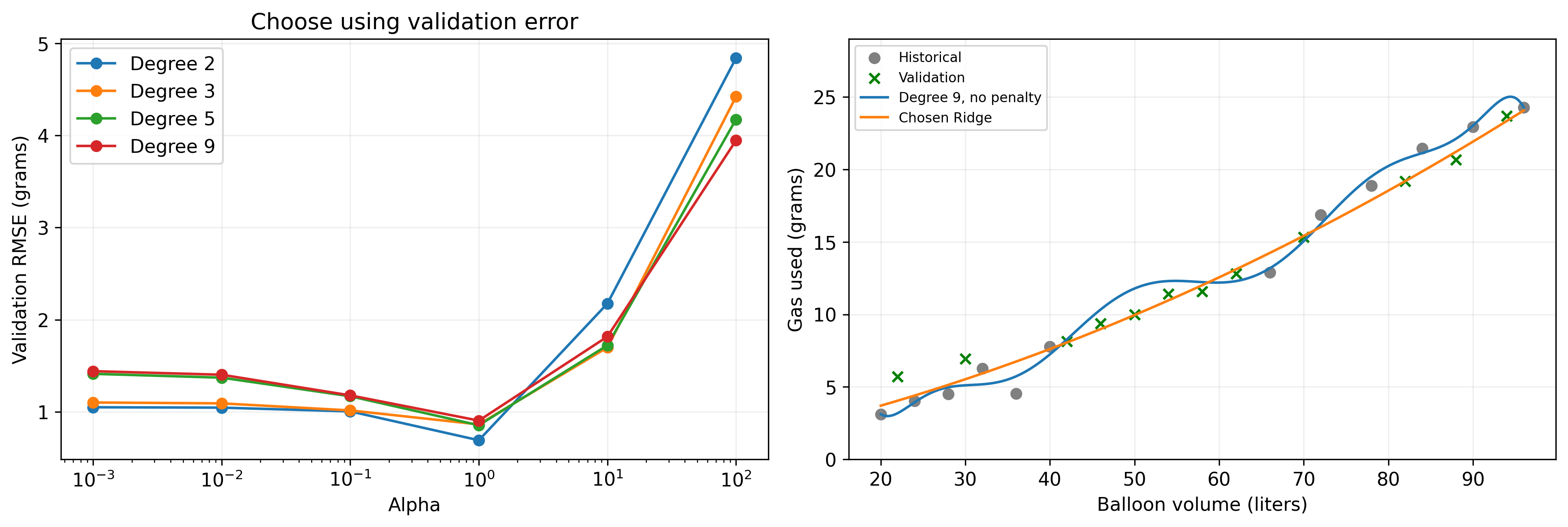
Use your Ridge function to fit each of the four degrees with alpha values of .001, .01, .1, 1, 10, and 100. Every fit uses the historical jobs. The supplied loop adds those models to the same collection as our line and unregularized curves.
We want to add our results to the candidates dict with their: {name, degree, alpha, and weights}.
Now compare all the candidates using validation RMSE and select the row with the lowest error. Store its model name and retrieve that candidate. There is just one winner, chosen from the whole table. If errors tie exactly, the supplied ordering keeps the first candidate.
Don't choose by historical error, and don't add the Ridge penalty to validation RMSE. At this point we're asking which model predicts new jobs most accurately.
Once you've selected a model, keep its weights, degree, and alpha fixed. Next we will open the mansion records. Those answers are for evaluating and interpreting the model, not choosing a different one.
Python Help
best_row = comparison.loc[comparison['validation_rmse'].idxmin()]
name = best_row['model']
Task 05-2: Code (0.5 pts.)
alphas = [.001, .01, .1, 1., 10., 100.]

# Re-running this cell should replace, rather than duplicate, Ridge candidates.
candidates = [candidate for candidate in candidates if candidate['alpha']==0]

for degree in degrees:
    for alpha in alphas:
        # TODO: Find the weights for our ridge regression
        weights = None

        # TODO: Add our candidate weights to our candidate list
        candidates.append(None)

comparison = compare_candidates(candidates)

# TODO: Get the best model out of the comparison results
best_row = None
selected_name = None

selected_model = next(candidate for candidate in candidates if candidate['name']==selected_name)

def predict_selected(x):
    return predict_candidate(selected_model, x)

print(comparison.sort_values('validation_rmse', kind='stable').to_string(
    index=False, float_format=lambda v: f'{v:.4f}'))

print(f'Chosen model: {selected_name}')
Task 05-2: Expected Output (0 pts.)
model  degree    alpha  historical_rmse  validation_rmse
    degree 2 Ridge (alpha=1)       2   1.0000           1.0459           0.6922
    degree 5 Ridge (alpha=1)       5   1.0000           1.2359           0.8551
    degree 3 Ridge (alpha=1)       3   1.0000           1.2798           0.8643
    degree 9 Ridge (alpha=1)       9   1.0000           1.1521           0.9054
  degree 2 Ridge (alpha=0.1)       2   0.1000           0.8497           1.0055
  degree 3 Ridge (alpha=0.1)       3   0.1000           0.8294           1.0161
 degree 2 Ridge (alpha=0.01)       2   0.0100           0.8472           1.0462
degree 2 Ridge (alpha=0.001)       2   0.0010           0.8472           1.0504
                    degree 2       2   0.0000           0.8472           1.0508
 degree 3 Ridge (alpha=0.01)       3   0.0100           0.8078           1.0927
degree 3 Ridge (alpha=0.001)       3   0.0010           0.8075           1.1020
                    degree 3       3   0.0000           0.8075           1.1031
  degree 5 Ridge (alpha=0.1)       5   0.1000           0.7123           1.1697
  degree 9 Ridge (alpha=0.1)       9   0.1000           0.7251           1.1793
               straight line       1   0.0000           1.0941           1.3153
                    degree 9       9   0.0000           0.5890           1.3416
 degree 5 Ridge (alpha=0.01)       5   0.0100           0.6799           1.3716
 degree 9 Ridge (alpha=0.01)       9   0.0100           0.6562           1.4034
degree 5 Ridge (alpha=0.001)       5   0.0010           0.6787           1.4131
                    degree 5       5   0.0000           0.6787           1.4186
degree 9 Ridge (alpha=0.001)       9   0.0010           0.6414           1.4419
   degree 3 Ridge (alpha=10)       3  10.0000           2.9167           1.6994
   degree 5 Ridge (alpha=10)       5  10.0000           2.9197           1.7225
   degree 9 Ridge (alpha=10)       9  10.0000           3.0438           1.8173
   degree 2 Ridge (alpha=10)       2  10.0000           3.6731           2.1761
  degree 9 Ridge (alpha=100)       9 100.0000           5.7772           3.9457
  degree 5 Ridge (alpha=100)       5 100.0000           6.1180           4.1737
  degree 3 Ridge (alpha=100)       3 100.0000           6.4558           4.4204
  degree 2 Ridge (alpha=100)       2 100.0000           7.0095           4.8394
Chosen model: degree 2 Ridge (alpha=1)
NOTE: Again the plot below is not part of your expected output.
Task 06-1: Description (0 pts.)
Taking Our Model Back to the Case
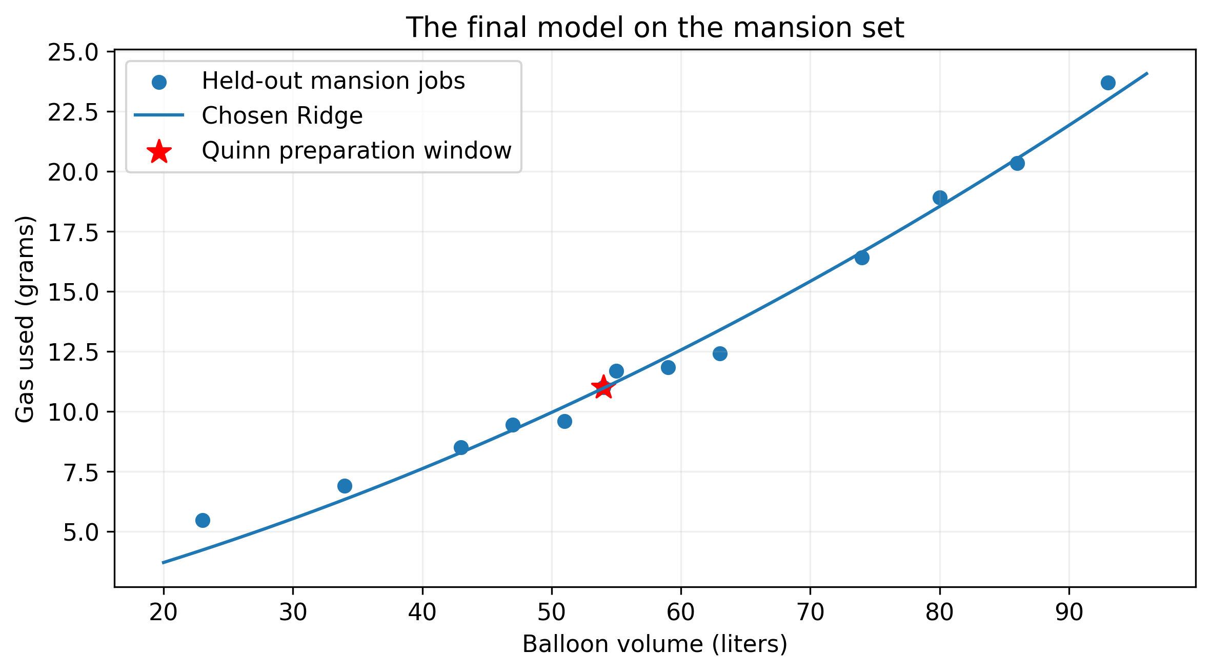
The mansion table contains thirteen balloon-filling jobs from the party preparations. We kept all of them out of fitting and model selection. Predict their gas use with your chosen model and calculate its RMSE.
One row, SCENE01, covers the canister in the kitchen and pantry from 19:55 to 20:45, overlapping Quinn's balloon preparations. The supplied code identifies that row. Calculate its measured gas use minus your prediction. A positive difference means more gas was used than expected.
The supplied comparison also shows what the degree-nine model without Ridge would have predicted for this job. Does the model that looked so impressive on the historical records lead us toward the same conclusion?
Keep your selected model fixed, even if a mansion result surprises you. We can report its errors honestly without changing our answer after seeing the test data.
Python Help
predictions = predict_selected(volumes)
error = rmse(measured, predictions)
difference = measured - predicted
Task 06-1: Code (0.5 pts.)
# TODO: Load the mansion.csv file
mansion_df = None
x_mansion = None
y_mansion = None

# TODO: Create predictions on our mansion (test) set
mansion_predictions = None
mansion_rmse = None

mansion_results = mansion_df.copy()
mansion_results['predicted_mass_loss_g'] = mansion_predictions

scene_index = mansion_df.index[mansion_df['trial_id']=='SCENE01'][0]
scene_measured = y_mansion[scene_index]
scene_prediction = mansion_predictions[scene_index]
scene_difference = scene_measured - scene_prediction

plain_nine = next(c for c in candidates if c['degree']==9 and c['alpha']==0)
plain_scene = predict_candidate(plain_nine, x_mansion[[scene_index]])[0]

print(mansion_results.to_string(index=False, float_format=lambda v: f'{v:.4f}'))
print(f'Chosen model: {selected_name}')
print(f'Mansion RMSE: {mansion_rmse:.4f} grams')
print(f"Quinn's preparation window: measured {scene_measured:.3f} g; predicted {scene_prediction:.3f} g")
print(f'Chosen-model unexplained difference: {scene_difference:.3f} g')
print(f'Degree-nine model without Ridge: predicted {plain_scene:.3f} g; difference {scene_measured-plain_scene:.3f} g')
Task 06-1: Expected Output (0 pts.)
trial_id  balloon_volume_liters  mass_loss_g  predicted_mass_loss_g
     R01                23.0000       5.4765                 4.2235
     R02                34.0000       6.9081                 6.3305
     R03                43.0000       8.5036                 8.2875
     R04                47.0000       9.4346                 9.2246
     R05                51.0000       9.5863                10.2032
     R06                55.0000      11.6934                11.2232
     R07                59.0000      11.8405                12.2846
     R08                63.0000      12.4135                13.3874
     R09                74.0000      16.4033                16.6339
     R10                80.0000      18.9101                18.5368
     R11                86.0000      20.3305                20.5330
     R12                93.0000      23.7009                22.9796
 SCENE01                54.0000      11.0120                10.9643
Chosen model: degree 2 Ridge (alpha=1)
Mansion RMSE: 0.5882 grams
Quinn's preparation window: measured 11.012 g; predicted 10.964 g
Chosen-model unexplained difference: 0.048 g
Degree-nine model without Ridge: predicted 12.301 g; difference -1.289 g
NOTE: The plot below still isn't part of your expected output.
Task 06-2: Short Answer Questions (0.5 pts.)
What Should We Tell Caulfield?
Use a few sentences for each answer.
Which unregularized degree fits the historical jobs most closely? Does it also have the lowest validation error? Explain what this tells you about overfitting.
[ANSWER]
Which model won the full validation comparison? Explain what Ridge changed and why we did not simply choose the lowest historical error.
[ANSWER]
Report the winner's mansion RMSE for
SCENE01. Compare that difference with the unregularized degree-nine prediction. Why must we keep our chosen model fixed after opening this set?[ANSWER]
Does ordinary balloon preparation seem to explain the gas use during Quinn's preparation window? What can these records tell us, and what additional evidence would you want before drawing a conclusion about Quinn?
[ANSWER]

Task 07-1: Description (0 pts.)
Sending in Your Report
Run the notebook from the beginning, save your work, and set GENERATE = True below to export your report. Make sure your written answers are included too! Colab will download the HTML; locally, run the export cell from the folder containing your saved notebook.
Task 07-1: Code (0 pts.)
GENERATE = False

NOTEBOOK_NAME = 'homework02.ipynb'

if GENERATE:
    import json
    from pathlib import Path
    import nbformat
    from nbconvert import HTMLExporter
    try:
        from google.colab import _message, files
    except ImportError:
        notebook_path = Path(NOTEBOOK_NAME)
        current = nbformat.read(notebook_path, as_version=4)
        in_colab = False
    else:
        notebook_path = Path('/content') / NOTEBOOK_NAME
        current = nbformat.reads(json.dumps(_message.blocking_request('get_ipynb', timeout_sec=10)['ipynb']), as_version=4)
        nbformat.write(current, notebook_path)
        in_colab = True
    html, _ = HTMLExporter().from_notebook_node(current)
    html_path = notebook_path.with_suffix('.html')
    html_path.write_text(html, encoding='utf-8')
    print(f'Exported {html_path.name}')
    if in_colab: files.download(str(html_path))
else:
    print('Export disabled. Set GENERATE = True when ready.')
Task 07-1: Reference Output (0 pts.)
Export disabled. Set GENERATE = True when ready.