Introduction to Artificial Intelligence - Homework Assignment 03 (5 pts.)
- Name:
- NETID:
Can We Trust the Witness?
Due September 28, 2026.
This assignment covers the following topics:
- Implementing the perceptron learning rule and training loop
- Connecting a weighted score to a decision boundary
- Logistic regression, sigmoid, and binary cross-entropy
- Comparing implementations and choosing a classification threshold
| Task | Description | Points |
|---|---|---|
| 00 | Prepare the witness records | 0.25 |
| 01 | Write and train a perceptron | 2.00 |
| 02 | Check the implementation and explain its limits | 0.50 |
| 03 | Write logistic predictions and loss | 1.00 |
| 04 | Compare thresholds on validation records | 0.50 |
| 05 | Evaluate and follow the mansion lead | 0.75 |
| 06 | Export the completed notebook | 0 |
| Total | 5.00 |
Run the cells in order and complete the written responses.
Story Progression
Caulfield has your report on the balloons and gas canisters. Quinn is still a lead, but the police need to look beyond one suspect's party supplies.
Fortunately, everyone at the mansion remembers something. Unfortunately, they do not remember the same something. A delivery, an argument, an envelope in the study—Caulfield has a stack of statements and time to follow only so many of them.
The department has records from earlier investigations. For each statement, officers checked some background details and interviewed the witness twice. Later, separate evidence established whether the main claim was corroborated. Can we learn from those earlier statements to help organize the new leads?
The intern suggests sorting by how confidently each witness spoke. Caulfield quietly takes the spreadsheet away from him.

Task 00: Prepare the Witness Records
Task 00-1: Description (0 pts.)
What Does One Row Mean?
Each row describes one statement, not a suspect. A person can be mistaken about one event and correct about another.
details_matched: how many of ten background details agreed with existing records, such as the room layout or the time dinner was served.details_repeated: how many of ten details stayed the same when the witness was interviewed again.corroborated:1if later, independent evidence supported the main claim;0if it contradicted it. Unresolved historical claims are excluded.
For example, a witness might repeat 6 of their 7 remembered details. Our input is [7, 6]. That does not tell us whether the envelope they described really existed: that is the separate claim we want to predict.
Which file should you use?
| File | Purpose | When to use it |
|---|---|---|
historical.csv |
Train the models | Start here |
validation.csv |
Choose a threshold | Before the final evaluation |
mansion_resolved.csv |
Evaluate separate mansion statements with resolved outcomes | Keep closed until Task 05 |
mansion_leads.csv |
Rank ongoing leads with no labels | Task 05; accuracy cannot be measured |
Task 00-1: Code (0 pts.)
import os
import shutil
import subprocess
from pathlib import Path

REPO_URL = 'https://github.com/wtheisen/nd-cse-30124-homeworks.git'

try:
    import google.colab
except ImportError:
    # Reuse a local checkout, including when launched from a homework subfolder.
    DATA_ROOT = next((p for p in [Path.cwd(), *Path.cwd().parents]
                      if (p / '.git').exists() and (p / 'evidence').is_dir()), None)
    if DATA_ROOT is None:
        DATA_ROOT = Path.cwd() / 'nd-cse-30124-homeworks'
else:
    # Leave the old checkout before deleting it, including on a setup-cell rerun.
    os.chdir('/content')
    DATA_ROOT = Path('/content/nd-cse-30124-homeworks')
    # Fetch fresh evidence every time this cell runs in Colab.
    if DATA_ROOT.exists():
        shutil.rmtree(DATA_ROOT)

if not DATA_ROOT.exists():
    subprocess.run(['git', 'clone', REPO_URL, str(DATA_ROOT)], check=True)

if not (DATA_ROOT / '.git').exists():
    raise RuntimeError(f'{DATA_ROOT} exists but is not a Git checkout. Choose a different clone location.')

# All later relative paths now start at the homework repository root.
os.chdir(DATA_ROOT)
DATA_ROOT = Path.cwd()

import numpy as np
import pandas as pd
from sklearn.linear_model import LogisticRegression
from sklearn.metrics import log_loss

EVIDENCE_DIR = DATA_ROOT / 'evidence' / 'homework03'
required_files = ['historical.csv', 'validation.csv', 'mansion_resolved.csv', 'mansion_leads.csv']
missing_files = [name for name in required_files if not (EVIDENCE_DIR / name).is_file()]
if missing_files:
    raise FileNotFoundError(
        f'HW03 evidence is missing: {missing_files}. '
        'In Colab, rerun setup after the evidence is released; locally, update this checkout with git pull --ff-only. '
    )

# Enter the evidence folder so the remaining cells can use simple filenames.
os.chdir(EVIDENCE_DIR)

FEATURES = ['details_matched', 'details_repeated']
historical_df = pd.read_csv('historical.csv')
validation_df = pd.read_csv('validation.csv')

print(historical_df.head().to_string(index=False))
print(f'Historical statements: {len(historical_df)}; validation statements: {len(validation_df)}')
Task 00-1: Expected Output (0 pts.)
statement_id  details_matched  details_repeated  corroborated
        H001                5                 5             0
        H002                5                 5             1
        H003                7                 7             1
        H004                0                 2             0
        H005                3                 9             1
Historical statements: 120; validation statements: 60
Task 00-2: Description (0 pts.)
[ME]: I've never heard the term "design matrix" before for the input with the column of 1s, where does that come from?
[ChatGPT]: Classical statistics—linear models, regression, and experimental design. The “design” refers to the experimental setup: the matrix encodes which treatments, conditions, or predictor values apply to each observation. It’s also common in econometrics. You’ll encounter it in statistically oriented ML treatments, but feature matrix or input matrix is more typical in modern ML/deep learning.
Reuse the Design Matrix
In HW02, a row of the design matrix started with 1 so the intercept could live inside the weight vector. We can use exactly the same trick here.
Build the input matrix in three steps:
- Select the two feature columns in the order shown above.
- Scale their counts by dividing by ten, so both range from zero to one.
- Prepend a column of ones for the bias.
For example: [8, 7] → [0.8, 0.7] → [1, 0.8, 0.7].
This is a fixed unit conversion, not a scaling rule learned from validation or test data.
Keep the original labels $y\in\{0,1\}$: 1 means corroborated and 0 means contradicted. Both the perceptron and logistic regression will use these same labels.
Python Help
features = df[['first_count', 'second_count']].to_numpy(dtype=float)
X = np.column_stack((np.ones(len(features)), features / 10.0))
Task 00-2: Code (0.25 pts.)
def make_design(df):
    # TODO: Select both feature columns and convert the counts to fractions.
    features = None
    # TODO: Add the intercept column, as in HW02.
    return None

X_train = make_design(historical_df)
X_val = make_design(validation_df)

# TODO: Extract the 0/1 labels for both classifiers.
y_train = None
y_val = None

print('Design matrix:', X_train.shape, '| labels:', y_train.shape)
print('Example [8, 7] becomes:', make_design(pd.DataFrame([[8, 7]], columns=FEATURES))[0])
Task 00-2: Expected Output (0 pts.)
Design matrix: (120, 3) | labels: (120,)
Example [8, 7] becomes: [1.  0.8 0.7]
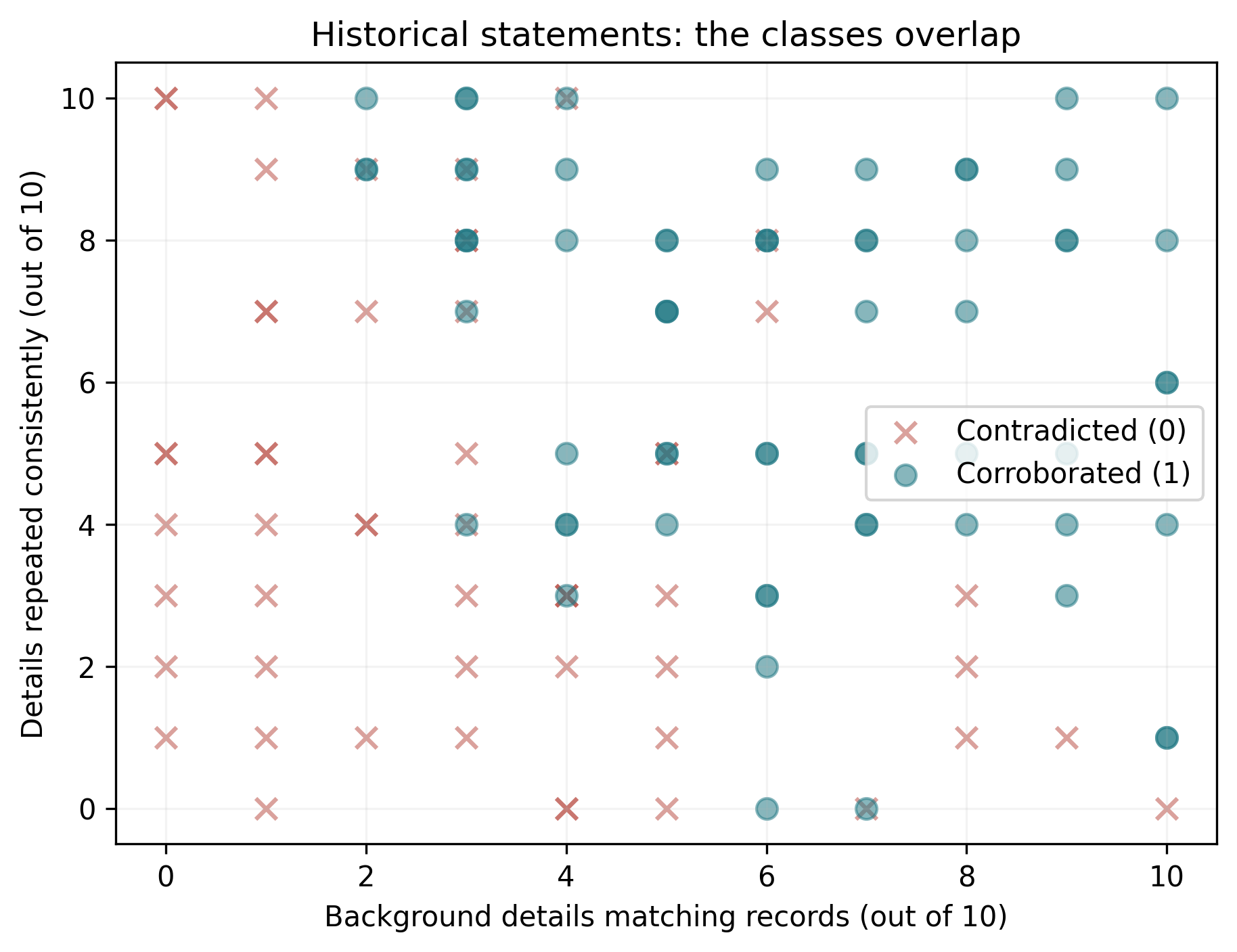
Figure 1. Both labels occur in the same region. Some points even share exactly the same two counts.
Task 01: Write and Train a Perceptron
Task 01-1: Description (0 pts.)
From a Number to a Class
HW02 predicted a quantity. Here we want a class. Start with the familiar weighted score:
$$s = Xw.$$
For one statement, that is $s=w_0+w_1x_1+w_2x_2$. Convert it to a class:
- Positive score ($s>0$): predict $\widehat{y}=1$.
- Zero or negative score ($s\leq 0$): predict $\widehat{y}=0$.
Use this same rule during training and evaluation, including an exact zero.
The set of points where $w_0+w_1x_1+w_2x_2=0$ is the decision boundary. With two features, it's a line. Moving the weights moves that line.
Return one 0/1 prediction per row. np.where(condition, value_if_true, value_if_false) is handy here. A score is not a probability: it can be negative or larger than one.
Task 01-1: Code (0.25 pts.)
def perceptron_predict(X, weights):
    # TODO: Compute scores and turn them into 0/1 predictions.
    scores = None

    return None

example_X = np.array([[1., 0., 0.], [1., .5, .5], [1., 1., 1.]])
example_w = np.array([-1., 1., 1.])

print('Scores:', example_X @ example_w)
print('Predictions:', perceptron_predict(example_X, example_w))
Task 01-1: Expected Output (0 pts.)
Scores: [-1.  0.  1.]
Predictions: [0 0 1]
Task 01-2: Description (0 pts.)
Learn from One Example
In HW02, sum of squared errors (SSE) used the difference between a true value and a prediction: $\sum_j(y_j-\widehat{y}_j)^2$. We will reuse that familiar target minus prediction error here. The true label $y$ and the perceptron's prediction $\widehat{y}$ are both 0 or 1, so $y-\widehat{y}$ can only be $-1$, $0$, or $+1$.
For each weight, apply the perceptron learning rule taught in class:
$$w_i' = w_i + \eta\,(y - \widehat{y})\,x_i.$$
The symbols mean:
- $\eta$ (Greek eta): the learning rate, with $\eta>0$.
- $i$: the feature index.
- $\widehat{y}$: the prediction from the current weights, computed before the update.
For the whole weight vector, the same rule is $w'=w+\eta\,(y - \widehat{y})\,x$.
| True label $y$ | Prediction $\widehat{y}$ | Error $y-\widehat{y}$ | Action |
|---|---|---|---|
| 1 | 0 | +1 | Add $\eta x$, increasing this example's score |
| 0 | 1 | -1 | Subtract $\eta x$, decreasing this example's score |
| 0 | 0 | 0 | Leave the weights unchanged |
| 1 | 1 | 0 | Leave the weights unchanged |
The first input is $x_0=1$, so the same rule updates the bias: $w_0'=w_0+\eta\,(y - \widehat{y})\,$. At a score of exactly zero, our prediction is 0: update if the true label is 1, and do nothing if it is 0.
The shared error term connects this rule to regression, but this is not gradient descent on SSE through the hard step function. The step function has zero derivative away from its threshold and is not differentiable at the threshold. We use the perceptron rule directly to correct classification mistakes.
Worked Example
Start with $w=[0,0,0]$, $x=[1,0.8,0.7]$, true label $y=1$, and learning rate $\eta=0.5$. The first input, $x_0=1$, is the bias input.
1. Compute the score using the current weights.
$$s=w_0x_0+w_1x_1+w_2x_2=(0)(1)+(0)(0.8)+(0)(0.7)=0.$$
2. Turn the score into a prediction.
Our rule predicts 1 only when $s>0$. Since $s=0$, the prediction is $\widehat{y}=0$.
3. Compute target minus prediction.
$$y-\widehat{y}=1-0=1.$$
4. Update each weight using that same error.
$$w_0'=w_0+\eta\,(y-\widehat{y})\,x_0=0+(0.5)(1)(1)=0.5.$$
$$w_1'=w_1+\eta\,(y-\widehat{y})\,x_1=0+(0.5)(1)(0.8)=0.4.$$
$$w_2'=w_2+\eta\,(y-\widehat{y})\,x_2=0+(0.5)(1)(0.7)=0.35.$$
Thus the new weight vector is $w'=[0.5,0.4,0.35]$. Compute the prediction and error once before updating any weights; do not recompute them between weight updates.
5. Check the new score for this example.
$$s'=(0.5)(1)+(0.4)(0.8)+(0.35)(0.7)=0.5+0.32+0.245=1.065.$$
The score is now positive, so the new prediction is 1, matching the true label.
What if the true label had been 0? Start again from the original weights $w=[0,0,0]$. The score is still zero and the prediction is still 0, but now the error is $y-\widehat{y}=0-0=0$. For every weight,
$$w_i'=w_i+\eta\,(0)\,x_i=w_i.$$
All three weights remain zero because the original prediction was already correct.
Your function should:
- Copy the weights so the caller's original array is preserved.
- Compute the prediction and error, then apply the update.
- Return the updated weights and a Boolean recording whether an update happened.
Task 01-2: Code (0.5 pts.)
def perceptron_step(x, target, weights, learning_rate):
    new_weights = weights.copy()

    # TODO: Compute the 0/1 prediction and target-minus-prediction error.
    prediction = None
    error = None

    # TODO: Apply the perceptron learning rule, including the bias.
    new_weights += None

    return new_weights, bool(error != 0)

step_w, changed = perceptron_step(np.array([1., .8, .7]), 1, np.zeros(3), .5)

print('New weights:', step_w, '| updated:', changed)
print('New score:', round(np.array([1., .8, .7]) @ step_w, 3))
Task 01-2: Expected Output (0 pts.)
New weights: [0.5  0.4  0.35] | updated: True
New score: 1.065
Task 01-3: Description (0 pts.)
Now Write the Training Loop
One example moves the boundary once. Training repeats that process across the dataset.
An epoch is one pass through every training example.
Before training: initialize the weights to zero and create an empty history.
For each epoch:
- Reset the update counter to zero.
- Visit the training rows in their given order.
- Update the weights for each row by calling your update function with that row and its label. Keep the returned weights and increment the counter if an update happened.
- Evaluate classification error across the training set using the final weights for this epoch.
- Record the epoch number, update count, and classification error in the history.
- Stop if the epoch made zero updates; otherwise begin the next epoch, up to
max_epochs.
Two measurements, two meanings:
- Update count: how often the weights changed during the pass.
- Classification error: how often the final weights predict incorrectly after the pass.
Why Might Training Keep Going?
The perceptron can converge on linearly separable data, but our witness records overlap. In particular, two historical rows have identical inputs and opposite labels. No deterministic classifier using just these inputs can classify both correctly. More epochs cannot remove that contradiction.
Training settings
- Learning rate:
1.0. - Maximum epochs:
40. - Row order: keep the given order; do not shuffle. A fixed order makes your implementation easier to check.
Return: the final weights and a list of history records containing epoch, updates, and error.
Python Help
for x, target in zip(X, targets):
    # x is one row, target is its matching label.
    pass
history.append({'epoch': epoch + 1, 'updates': updates, 'error': error})

Task 01-3: Code (1.25 pts.)
def train_perceptron(X, targets, learning_rate=1.0, max_epochs=40):
    weights = np.zeros(X.shape[1], dtype=float)
    history = []

    for epoch in range(max_epochs):
        updates = 0

        for x, target in zip(X, targets):
            # TODO: Step through examples and labels, keeping each new weight vector.
            weights, changed = None

            updates += int(changed)

        # TODO: Measure classification error after the full pass.
        error = None

        history.append({'epoch': epoch + 1, 'updates': updates, 'error': float(error)})

        # TODO: Stop if a complete pass needed no updates. (~2 lines)
        pass

    return weights, history

perceptron_w, training_history = train_perceptron(X_train, y_train)
history_df = pd.DataFrame(training_history)

print(history_df.iloc[[0, 1, 4, -1]].to_string(index=False))
print('Final weights:', np.round(perceptron_w, 4))
print(f'Validation accuracy: {np.mean(perceptron_predict(X_val, perceptron_w) == y_val):.3f}')
Task 01-3: Reference Output (0 pts.)
epoch  updates    error
     1       50 0.233333
     2       35 0.341667
     5       30 0.183333
    40       36 0.266667
Final weights: [-3.   4.4  1.3]
Validation accuracy: 0.767
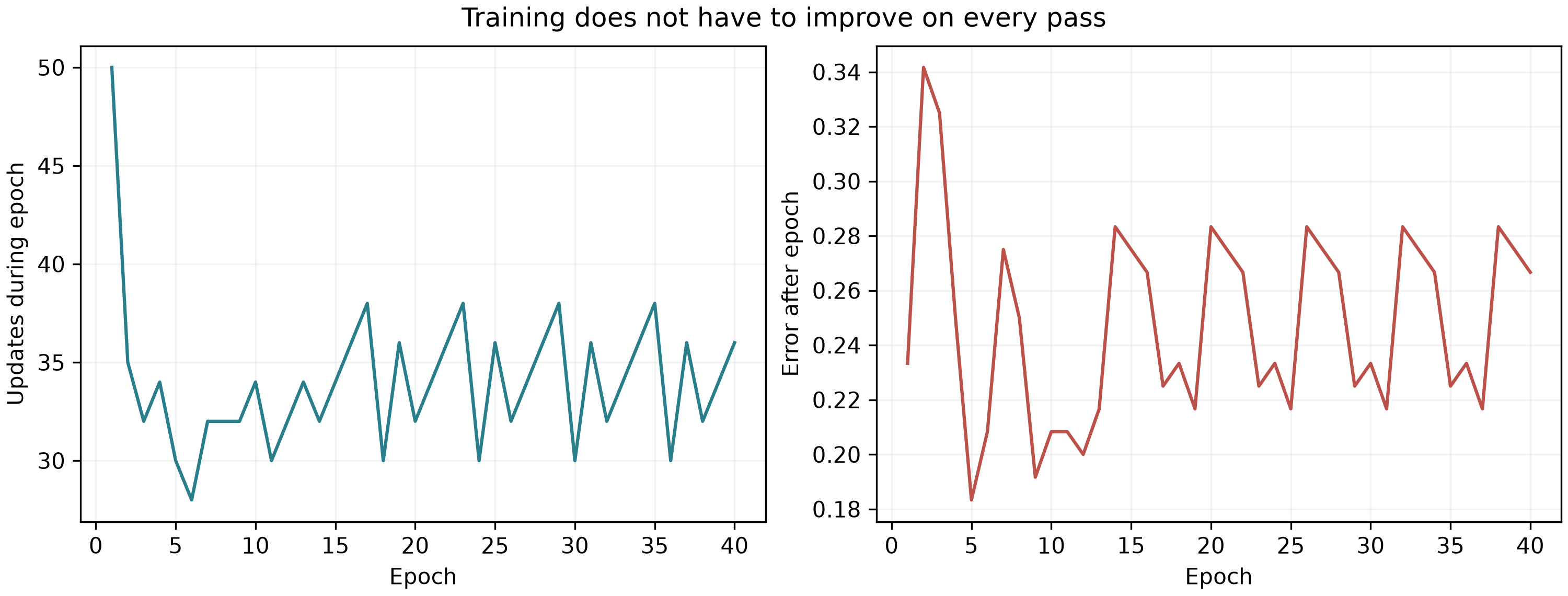
Figure 2. The update count and the final error describe different things. Neither is guaranteed to fall every epoch.
Task 02: Check the Perceptron
Task 02-1: Description (0 pts.)
Check Against Hand Calculations
Check the update on examples whose answers you can calculate yourself. With $x=[1,0.8,0.7]$ and a learning rate of 0.5, a missed positive adds [0.5,0.4,0.35], a false positive subtracts it, and a correct prediction leaves the weights unchanged.
Complete the call to your update function. The six supplied cases cover both mistakes, both correct predictions, and both labels at a score of exactly zero.
The assertions check that:
- The updated weights match the hand calculation.
- The update flag is correct.
- The original weights were preserved.
A separate tiny dataset checks the full training loop and early stopping.
We use explicit hand calculations rather than requiring identical weights from scikit-learn. Its perceptron updates on a zero signed margin for either label, while our class rule predicts 0 at zero and updates only on mistakes. Different tie behavior can produce different training trajectories.
Task 02-1: Code (0.25 pts.)
# Supplied hand-calculated cases: (starting weights, target, expected weights, updated).
x_check = np.array([1., .8, .7])

check_cases = [
    ([-1., 0., 0.], 1, [-.5, .4, .35], True),   # missed positive
    ([1., 0., 0.], 0, [.5, -.4, -.35], True),   # false positive
    ([-1., 0., 0.], 0, [-1., 0., 0.], False),  # correct negative
    ([1., 0., 0.], 1, [1., 0., 0.], False),    # correct positive
    ([0., 0., 0.], 1, [.5, .4, .35], True),    # zero score, positive target
    ([0., 0., 0.], 0, [0., 0., 0.], False),   # zero score, negative target
]

for initial, target, expected, expected_changed in check_cases:
    original = np.array(initial)

    # TODO: Run one update for this example with learning rate 0.5.
    actual, changed = None
    np.testing.assert_allclose(actual, expected, atol=1e-12)
    assert changed == expected_changed
    np.testing.assert_array_equal(original, initial)

print('Six hand-calculated update checks passed.')

# Supplied check: these two points can be separated, so training should stop early.
toy_X = np.array([[1., 0.], [1., 1.]])
toy_y = np.array([0, 1])
toy_w, toy_history = train_perceptron(toy_X, toy_y, max_epochs=10)
np.testing.assert_array_equal(toy_w, [0., 1.])
np.testing.assert_array_equal(perceptron_predict(toy_X, toy_w), toy_y)
assert [row['updates'] for row in toy_history] == [1, 1, 0]
assert toy_history[-1]['error'] == 0.0
print('Training-loop and early-stopping checks passed.')
Task 02-1: Expected Output (0 pts.)
Six hand-calculated update checks passed.
Training-loop and early-stopping checks passed.
Task 02-2: Written Response (0.25 pts.)
Why does the positive example in Task 01-2 increase its own score after the update?
[ANSWER]
Would raising
max_epochsguarantee zero training error on these witness records? Explain using the two identical inputs.[ANSWER]
Story Progression
Your implementation passes the hand-calculated checks. Caulfield looks pleased until the intern points out that every statement still gets the same two possible answers: yes or no.
Two claims can both land on the positive side of the line even when one is barely across it. Could we get something more informative than a hard decision?

Task 03: Logistic Regression
Task 03-1: Description (0 pts.)
Same Score, Different Output
Logistic regression also starts with $s=Xw$. It passes that score through the sigmoid:
$$\sigma(s)=\frac{1}{1+e^{-s}}.$$
A score of zero becomes 0.5. Positive scores produce probabilities above 0.5, and negative scores produce probabilities below it. Despite its name, logistic regression is a classification model here.
Implement the prediction in two steps:
- Write
sigmoidto transform scores into probabilities. - In
predict_probability, computeX @ weightsand pass those scores through your sigmoid function.
Return one probability per statement. We'll interpret it as the model's estimated probability of corroboration—not a measured probability that someone is telling the truth.
For numerical stability, the supplied split handles positive and negative scores separately. For negative $s$, the equivalent expression $e^s/(1+e^s)$ avoids computing a huge $e^{-s}$. Fill the nonnegative-score expression. The negative-score expression, masks, and allocation are supplied.
Task 03-1: Code (0.5 pts.)
def sigmoid(scores):
    scores = np.asarray(scores, dtype=float)
    result = np.empty_like(scores)
    positive = scores >= 0

    # TODO: Apply sigmoid to nonnegative scores.
    result[positive] = None

    exp_scores = np.exp(scores[~positive])

    result[~positive] = exp_scores / (1.0 + exp_scores)

    return result

def predict_probability(X, weights):
    # TODO: Pass the weighted score through your sigmoid function.
    return None

print('Sigmoid([-2, 0, 2]):', np.round(sigmoid(np.array([-2., 0., 2.])), 4))
print('Extreme-score check:', sigmoid(np.array([-1000., 1000.])))
Task 03-1: Expected Output (0 pts.)
Sigmoid([-2, 0, 2]): [0.1192 0.5    0.8808]
Extreme-score check: [0. 1.]
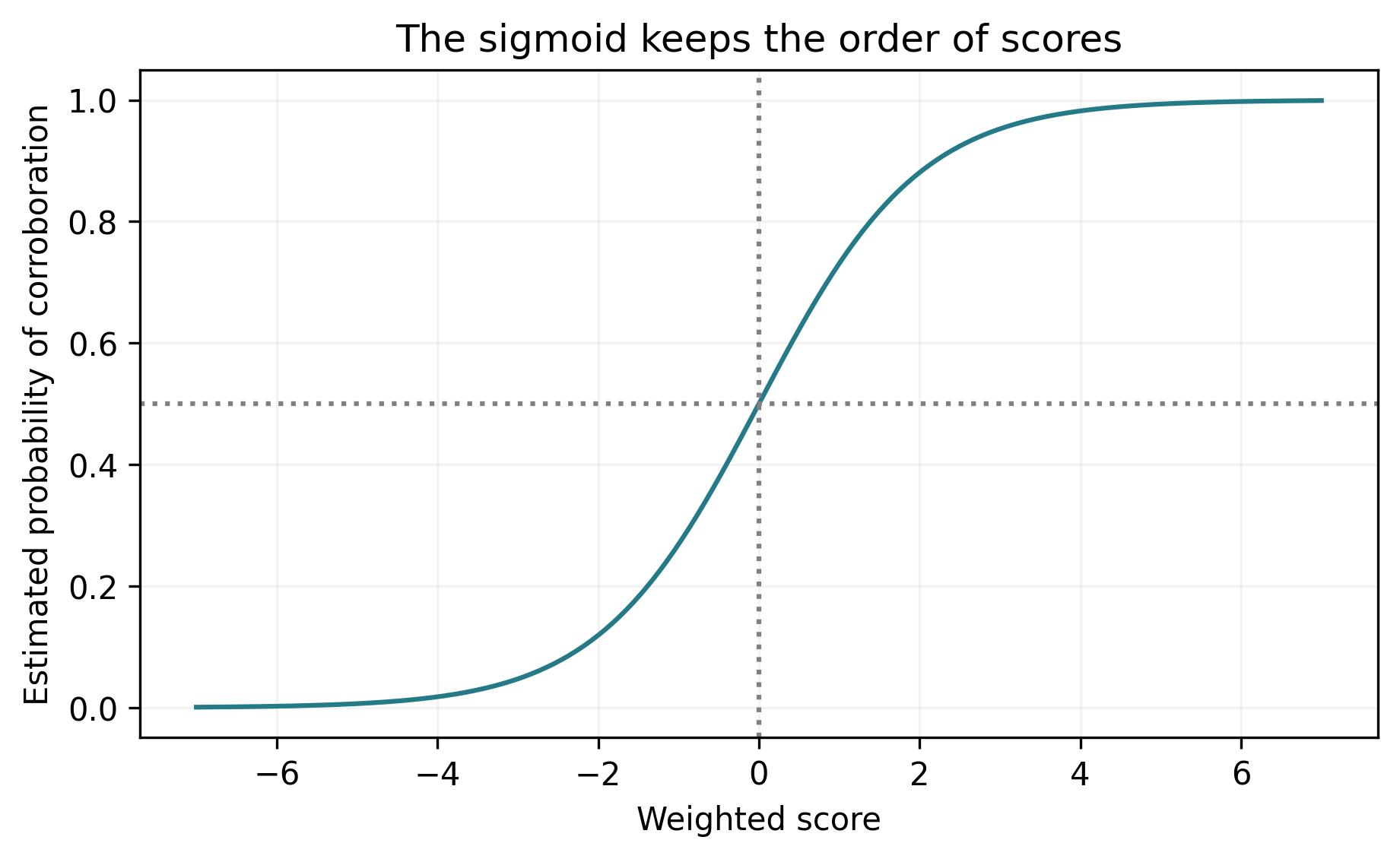
Figure 3. Sigmoid changes the output scale. It does not turn a linear boundary into a curved one.
Task 03-2: Description (0 pts.)
How Wrong Was That Probability?
Accuracy treats 0.51 and 0.99 the same when both predict class 1. A loss for probabilities should notice the difference—especially when the answer is actually 0.
For labels $y\in\{0,1\}$ and probabilities $p$, binary cross-entropy is
$$L=-\frac{1}{n}\sum_{i=1}^{n}\left[y_i\log(p_i)+(1-y_i)\log(1-p_i)\right].$$
When $y=1$, only $-\log(p)$ remains. Predicting 0.9 costs about 0.105; predicting 0.1 costs about 2.303. Confident mistakes receive a much larger penalty.
To implement the loss:
- Clip probabilities to
[1e-12, 1-1e-12]so rounding to zero or one does not causelog(0). - Compute both terms using
np.log, the natural logarithm. - Take the negative mean across examples.
Task 03-2: Code (0.5 pts.)
def binary_cross_entropy(y, probabilities):
    p = np.clip(probabilities, 1e-12, 1.0 - 1e-12)

    # TODO: Compute and average both terms of binary cross-entropy.
    return None

print(f'Correct and confident: {binary_cross_entropy(np.array([1]), np.array([.9])):.3f}')
print(f'Wrong and confident:   {binary_cross_entropy(np.array([1]), np.array([.1])):.3f}')
print(f'Always 0.5:            {binary_cross_entropy(y_val, np.full(len(y_val), .5)):.3f}')
Task 03-2: Expected Output (0 pts.)
Correct and confident: 0.105
Wrong and confident:   2.303
Always 0.5:            0.693
Task 03-3: Description (0 pts.)
Let the Library Fit the Weights
We wrote the perceptron's training loop ourselves. For logistic regression, the library will fit the weights. Its solver repeatedly adjusts them to reduce the loss; we will implement gradient-based network training in HW07.
The perceptron updates only when its 0/1 prediction is wrong. Logistic fitting also responds to how confident predictions are. The two procedures need not find the same line.
Create and fit the library model:
- Construct a
LogisticRegressionmodel using all the settings below. - Fit it to
X_trainandy_trainbefore accessingcoef_[0].
Required settings:
solver='lbfgs': an iterative optimizer. You do not need to implement this solver.C=np.inf: disables regularization in the supplied scikit-learn version, leaving binary cross-entropy as the objective.fit_intercept=False: the intercept is already included inside $X$.max_iter=2000andtol=1e-10: allow sufficient iterations and use the specified stopping tolerance.
The solver uses a different procedure from our perceptron update rule.
After fitting, the supplied assertions compare your probabilities and cross-entropy with scikit-learn. They stop execution if the calculations disagree; the success message appears only after both checks pass. This verifies the forward calculation and loss, not the library's optimizer.
This model-fitting step is required setup and carries no separate points.
Task 03-3: Code (0 pts.)
# TODO: Construct LogisticRegression with C=np.inf, fit_intercept=False,
# solver='lbfgs', max_iter=2000, and tol=1e-10, then fit it to X_train and y_train.
logistic_model = None

logistic_w = logistic_model.coef_[0]
p_val = predict_probability(X_val, logistic_w)

# Supplied checks for your probability and loss implementations.
np.testing.assert_allclose(
    p_val, logistic_model.predict_proba(X_val)[:, 1], atol=1e-10
)
np.testing.assert_allclose(
    binary_cross_entropy(y_val, p_val), log_loss(y_val, p_val), atol=1e-10
)

print('Probability and loss checks passed.')
print('Logistic weights:', np.round(logistic_w, 4))
print(f'Validation cross-entropy: {binary_cross_entropy(y_val, p_val):.3f}')
print(f'Validation accuracy at 0.5: {np.mean((p_val >= .5) == y_val):.3f}')
Task 03-3: Reference Output (0 pts.)
Probability and loss checks passed.
Logistic weights: [-5.4055  6.8752  4.6096]
Validation cross-entropy: 0.457
Validation accuracy at 0.5: 0.800
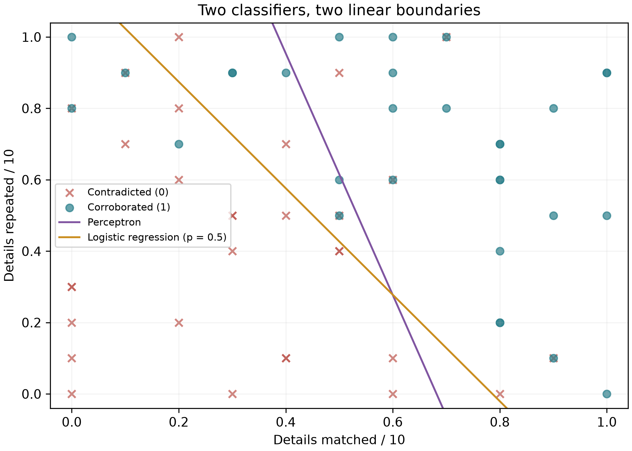
Figure 4. Both boundaries are straight lines. These points are validation records; circles were corroborated and crosses contradicted.
Task 04: Choose a Follow-up Threshold
Task 04-1: Description (0 pts.)
Who Goes on the Follow-up List?
A probability does not choose an action for us. We need a threshold: follow up when $p\geq\tau$.
Four Possible Outcomes
- Positive means the model predicts “follow up”; negative means “skip.”
- True means the prediction is correct; false means it is incorrect.
Read the actual outcome down the rows and the model prediction across the columns:
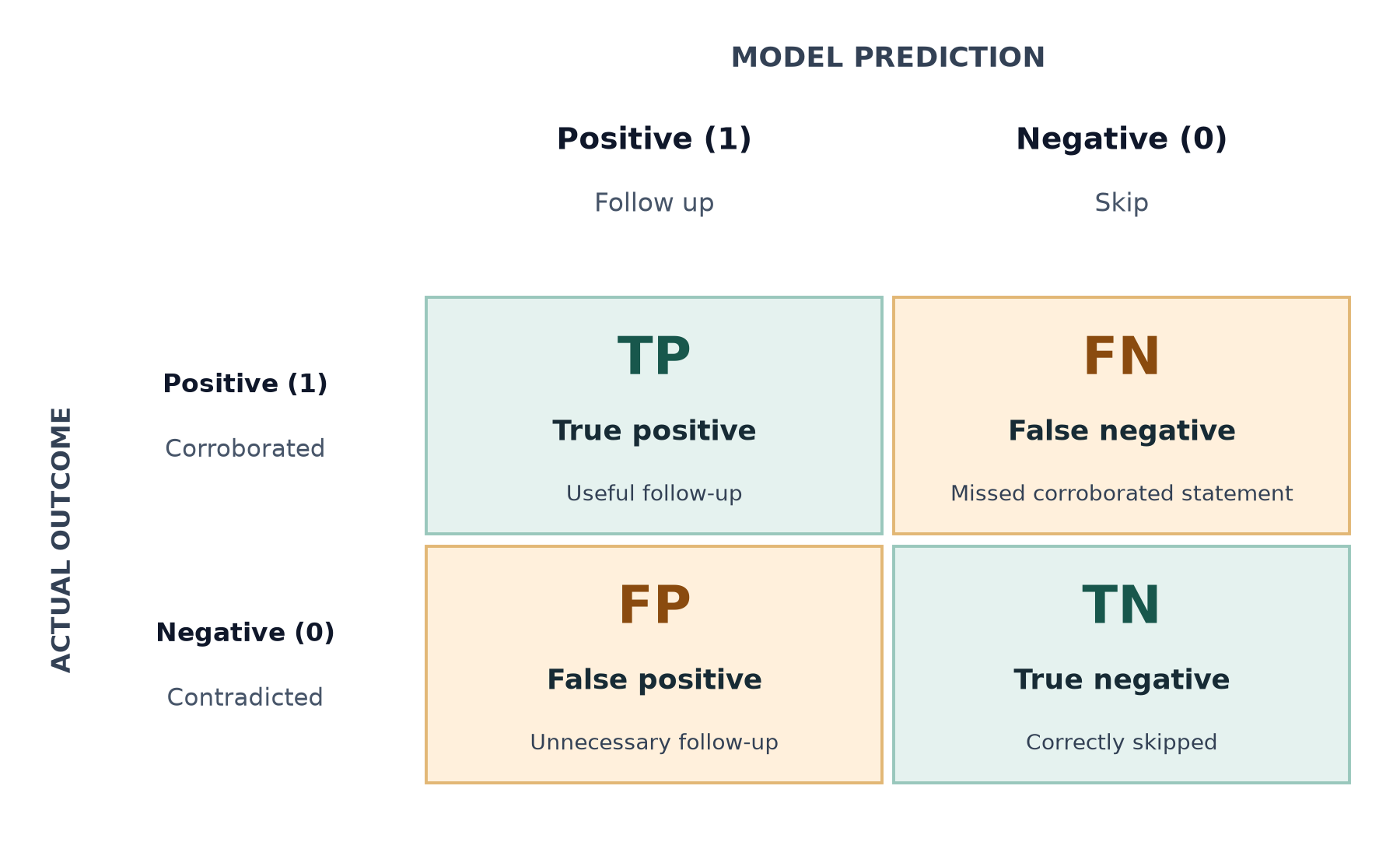
For example, following up on a statement that was actually contradicted is a false positive. Skipping one that was corroborated is a false negative.
Each statement belongs in one box. The counts in these four boxes form a confusion matrix.
Count the Costs
Caulfield wants to avoid missing a useful lead, but interviews also take time. For this exercise, he counts a missed corroborated statement as two mistakes and an unnecessary follow-up as one. On validation records, choose among thresholds 0.3, 0.5, and 0.7 by minimizing
$$\text{cost}=2\,\text{false negatives}+\text{false positives}.$$
These are screening decisions, not accusations. The model's weights stay fixed while we change the threshold.
Threshold selection procedure:
- Convert probabilities into predictions for each candidate threshold.
- Count false positives and false negatives on the validation records.
- Calculate the cost and select the threshold with the lowest cost.
- If costs tie, choose the higher threshold, giving a smaller follow-up list.
- Freeze that choice before opening the mansion outcomes.
Implement the predictions and both error counts. The loop and selection are supplied.
Python Help
count = np.sum((predictions == 1) & (labels == 0))
Parentheses around each comparison are necessary when combining NumPy conditions with &.

Task 04-1: Code (0.5 pts.)
def threshold_report(y, probabilities, threshold):
    # TODO: Convert probabilities into 0/1 follow-up decisions.
    predictions = None

    # TODO: Count false positives and false negatives separately.
    fp = None
    fn = None

    return {'threshold': threshold, 'follow_ups': int(predictions.sum()),
            'false_positives': fp, 'false_negatives': fn, 'cost': 2*fn + fp,
            'accuracy': float(np.mean(predictions == y))}

threshold_table = pd.DataFrame([threshold_report(y_val, p_val, t) for t in [.3, .5, .7]])
selected = threshold_table.sort_values(['cost', 'threshold'], ascending=[True, False]).iloc[0]
selected_threshold = float(selected['threshold'])

print(threshold_table.to_string(index=False, float_format=lambda x: f'{x:.3f}'))
print(f'Frozen threshold: {selected_threshold:.1f}')
Task 04-1: Reference Output (0 pts.)
threshold  follow_ups  false_positives  false_negatives  cost  accuracy
     0.300          43               14                1    16     0.750
     0.500          34                8                4    16     0.800
     0.700          26                4                8    20     0.800
Frozen threshold: 0.5
Task 05: Return to the Mansion
Task 05-1: Description (0 pts.)
One Final Check, Then the New Leads
First, evaluate the resolved statements:
- Open
mansion_resolved.csv. - Evaluate both models, keeping every weight and the selected threshold fixed.
- Compare classification accuracy.
- For logistic regression, also report cross-entropy and the missed/extra follow-ups.
We do not need logistic regression to win every metric for probabilities to be useful.
Then, rank the unresolved leads:
- Open
mansion_leads.csvand compute an estimated probability for each lead. - Rank the leads by that probability.
- Flag leads that meet the frozen follow-up threshold.
These leads have no known answers. The statement text and its ID are for Caulfield to read; neither is a model feature.
Complete the marked prediction lines. The loading and report formatting are supplied. A high rank tells us where the model would start an investigation, not how the investigation will end.
Task 05-1: Code (0.25 pts.)
mansion_df = pd.read_csv('mansion_resolved.csv')
X_mansion = make_design(mansion_df)
y_mansion = mansion_df['corroborated'].to_numpy(dtype=int)

# TODO: Evaluate the fixed perceptron and logistic model on the mansion set.
perceptron_mansion = None
p_mansion = None

print(f'Perceptron mansion accuracy: {np.mean(perceptron_mansion == y_mansion):.3f}')
print(f'Logistic mansion accuracy at 0.5: {np.mean((p_mansion >= .5) == y_mansion):.3f}')
print(f'Logistic mansion cross-entropy: {binary_cross_entropy(y_mansion, p_mansion):.3f}')
print('Frozen-threshold report:', threshold_report(y_mansion, p_mansion, selected_threshold))

leads_df = pd.read_csv('mansion_leads.csv')

# TODO: Score the unresolved leads with the same weights and threshold and find witness follow ups
leads_df['estimated_probability'] = None
leads_df['follow_up'] = None

ranked_leads = leads_df.sort_values(['estimated_probability', 'statement_id'], ascending=[False, True])

print(ranked_leads[['statement_id', 'estimated_probability', 'follow_up']].to_string(index=False, float_format=lambda x: f'{x:.3f}'))
print('Highest-ranked statement:', ranked_leads.iloc[0]['statement'])
Task 05-1: Reference Output (0 pts.)
Perceptron mansion accuracy: 0.750
Logistic mansion accuracy at 0.5: 0.683
Logistic mansion cross-entropy: 0.497
Frozen-threshold report: {'threshold': 0.5, 'follow_ups': 33, 'false_positives': 15, 'false_negatives': 4, 'cost': 23, 'accuracy': 0.6833333333333333}
statement_id  estimated_probability  follow_up
         L02                  0.993       True
         L04                  0.898       True
         L06                  0.736       True
         L05                  0.471      False
         L03                  0.469      False
         L01                  0.066      False
Highest-ranked statement: A catering assistant heard a guest addressed as Professor Dingler. He carried an envelope into the study and left it in the desk drawer.
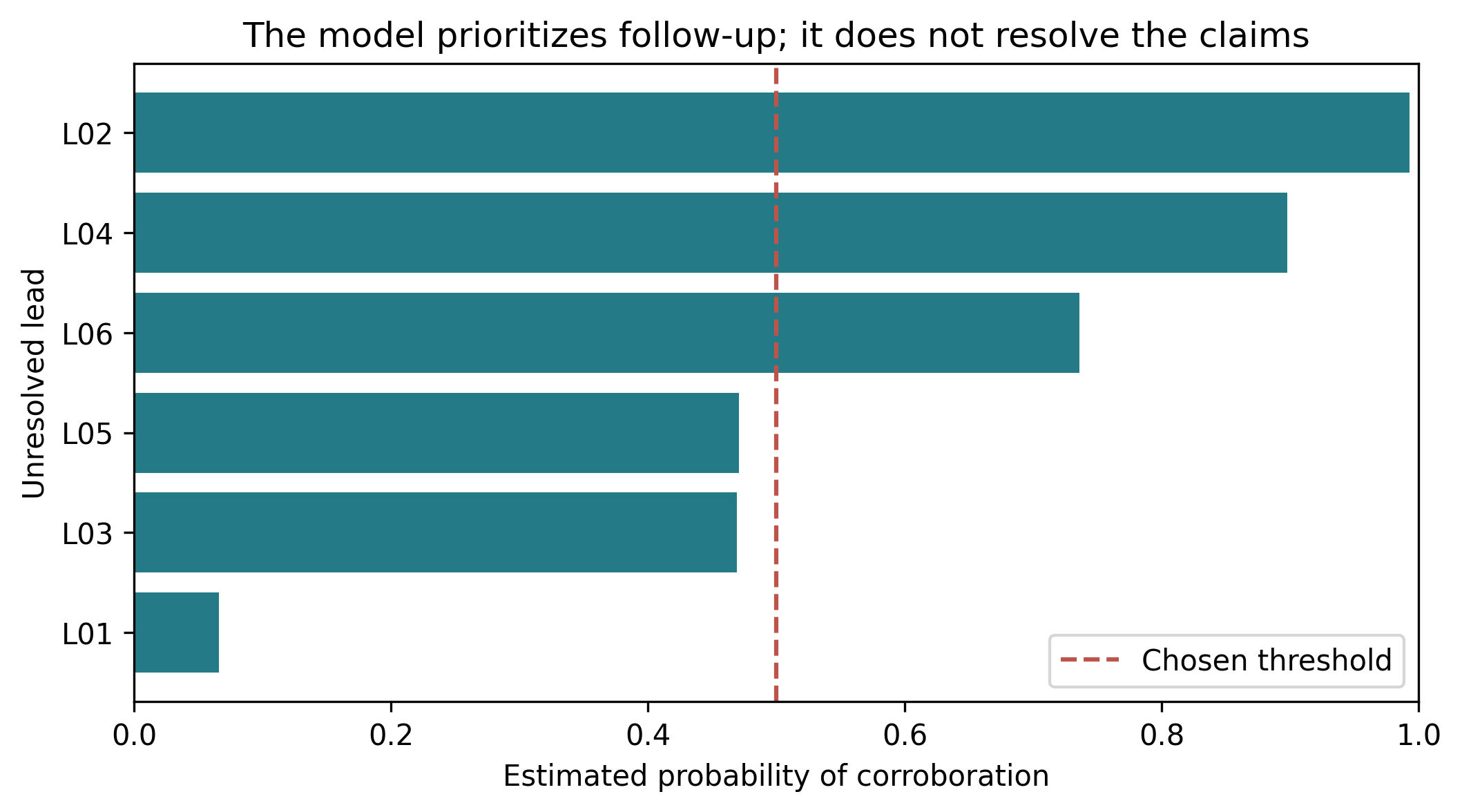
Figure 5. L02 is the highest-ranked lead. The dashed line is the threshold selected on validation records.
Task 05-2: Written Response (0.50 pts.)
Compare thresholds
0.3and0.5on the validation records. How many false positives and false negatives does each produce? Show why their costs tie under $\text{cost}=2\,\text{false negatives}+\text{false positives}$. Which threshold does our tie-breaking rule select, and what tradeoff does that choice make?[ANSWER]
Report both models' mansion accuracies at their stated thresholds and logistic cross-entropy. Why would changing settings after seeing those results spoil the held-out check?
[ANSWER]
Which unresolved lead ranked first? Explain what the probability estimates and name one piece of new evidence Caulfield should seek.
[ANSWER]
Does sigmoid give logistic regression a nonlinear decision boundary in our two original features? Explain.
[ANSWER]
Story Progression
The highest-ranked statement gives Caulfield a name: Professor Dingler.
The catering assistant remembers Dingler carrying an envelope into the study and leaving it in a desk drawer. Caulfield follows the lead and finds the envelope there. Inside are several letters. Now we have a physical piece of evidence to examine, rather than another score in a spreadsheet.

The forensics team scans the pages. The intern volunteers to organize the image files.
By the time Caulfield asks for them, the scans have been scrambled and their colors are wrong. The pixels are still there. The readable letters are not.
That is where HW04 begins: recovering the damaged letter images associated with Professor Dingler. For now, file your witness report—and perhaps keep the intern away from the originals.

Task 06: Export the Completed Notebook
Task 06-1: Description (0 pts.)
- Complete and run your code, and include your name, NETID, and written responses.
- Save the notebook. For local execution, make sure
NOTEBOOK_NAMEmatches your saved filename inhomeworks/homework03/. - Set
GENERATE = Truebelow and run the export cell. - Open the HTML file and check that your answers and outputs are present before submitting it.
In Colab, the cell captures the current notebook and downloads the HTML submission file. Locally, it reads the saved notebook and writes the HTML beside it. Exporting includes existing outputs; it does not rerun your solutions.
Task 06-1: Code (0 pts.)
GENERATE = False
NOTEBOOK_NAME = 'homework03.ipynb'

if GENERATE:
    import json
    from pathlib import Path
    import nbformat
    from nbconvert import HTMLExporter

    try:
        from google.colab import _message, files
    except ImportError:
        notebook_path = DATA_ROOT / 'homeworks/homework03' / NOTEBOOK_NAME
        current = nbformat.read(notebook_path, as_version=4)
        in_colab = False
    else:
        notebook_path = Path('/content') / NOTEBOOK_NAME
        snapshot = _message.blocking_request('get_ipynb', timeout_sec=30)
        current = nbformat.reads(json.dumps(snapshot['ipynb']), as_version=4)
        nbformat.write(current, notebook_path)
        in_colab = True

    # Figures use the course's hosted image URLs.
    notebook_folder = DATA_ROOT / 'homeworks/homework03'
    exporter = HTMLExporter()
    exporter.embed_images = False
    html, _ = exporter.from_notebook_node(
        current, resources={'metadata': {'path': str(notebook_folder)}}
    )
    html_path = notebook_path.with_suffix('.html')
    html_path.write_text(html, encoding='utf-8')
    print(f'Exported {html_path.name}')
    if in_colab:
        files.download(str(html_path))
    else:
        print(f'Saved to: {html_path}')
else:
    print('Export disabled. Set GENERATE = True when ready.')
Task 06-1: Expected Output (0 pts.)
Export disabled. Set GENERATE = True when ready.
With GENERATE = True, the cell reports the exported filename and, in Colab, starts the download.