Introduction to Artificial Intelligence - Homework Assignment 06 (5 pts.)
- Name:
- NETID:
Teaching the Computer to Look Due November 2, 2026.
This assignment covers:
- Turning images into tensors, batches, and flattened feature vectors
- Implementing an affine (linear) layer and choosing an initial weight scale
- Why neural networks need nonlinear activations such as ReLU
- Turning logits into probabilities and a numerically stable cross-entropy loss
- Assembling a feed-forward network and checking it against PyTorch
| Task | Description | Points |
|---|---|---|
| 00 | Load the character evidence | 0.25 |
| 01 | Turn images into tensors and batches | 0.75 |
| 02 | Build an affine layer; explain the initialization | 0.875 |
| 03 | Add a nonlinearity; explain the collapse | 0.375 |
| 04 | Turn logits into a stable loss; interpret the chance loss | 1.125 |
| 05 | Assemble the network | 0.50 |
| 06 | Check against PyTorch and inspect the predictions | 0.75 |
| 07 | Report the results to Caulfield | 0.375 |
| 08 | Export the notebook | 0 |
| Total | 5.00 |
Run the cells in order and answer the written questions. This assignment uses PyTorch but does not train anything: every network you build this week keeps its random starting weights. In HW07, we will teach it.
Story Progression
Caulfield finally has readable pages, and your SVM tells him where the cut-out letters sit. That leaves a few hundred characters that still need to be read. The intern volunteered to read them all by hand, then asked whether the squiggly one was a "2" or a "Z". Caulfield would like a second opinion that doesn't drink his coffee.
The forensics lab keeps a reference archive of 9,400 handwritten characters, each already labeled by an analyst. There are 47 possible labels: ten digits, all 26 uppercase letters, and the 11 lowercase letters that don't look like their uppercase versions. If we can build a model that learns from this archive, we can point it at the recovered evidence.
This week we will build the forward pass of a feed-forward neural network: the calculation that turns a 28 × 28 image into one score per character. HW02 gave us a linear model for one number. HW03 gave us a linear model for two classes. Now we will stack several linear layers, add nonlinearities between them, and produce 47 class scores at once.
Our network will start with random weights, so its first guesses will be terrible. That is expected. This week we make sure the calculation is correct; in HW07, we make it accurate.
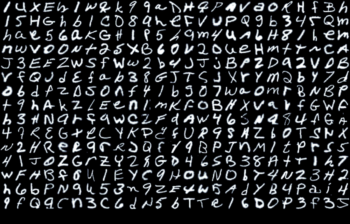
Task 00: Load the Character Evidence
Task 00-1: Description (0 pts.)
What Is in the Archive?
The archive is a balanced subset of EMNIST, the "extended" version of the classic MNIST handwritten-digit dataset. Every example is one 28 × 28 grayscale image of a single character:
- Each pixel is an unsigned 8-bit integer (
uint8) from0(black background) to255(bright ink). - Each label is an integer class ID from
0to46.classes.jsonmaps those IDs back to characters: ID10meansA, ID36meansa, and so on.
Why only 11 lowercase letters? EMNIST's "balanced" split merges lowercase letters that are hard to tell apart from their uppercase versions when handwritten. A handwritten c and C are usually the same shape at a different size, so both are labeled C. The letters that stay separate (a b d e f g h n q r t) look different from their capitals. Keep this in mind when you inspect mistakes: some errors are genuinely ambiguous, even for a person.
| File | Contents | When to use it |
|---|---|---|
emnist_balanced_small_train.npz |
X: (9400, 28, 28) images, y: (9400,) labels |
Now: we split it into training and validation sets |
emnist_balanced_small_test.npz |
2,350 held-out images and labels | Keep closed until HW07's final comparison |
classes.json |
The ordered list of 47 class names | Translating IDs into characters |
The files already use the course's image orientation. Do not transpose or rotate them. (The raw EMNIST download is stored sideways; we've already fixed that.)
Your Task
The setup code loads the arrays for you. Complete one line:
- Count how many examples belong to each class with
np.bincount. Passminlength=len(classes)so a missing class would still appear as a zero.
The supplied code prints the counts, the first few labels, and a grid with one example of each class. A balanced dataset should have the same count for every class. Look closely at the printed labels: the file stores all 200 examples of one class, then all 200 of the next. That ordering will matter in Task 01.
Python Help
labels = np.array([0, 2, 2, 1, 2])
np.bincount(labels)               # array([1, 1, 3]): one 0, one 1, three 2s
np.bincount(labels, minlength=5)  # array([1, 1, 3, 0, 0])
Useful Links
Task 00-1: Code (0.25 pts.)
import os
import shutil
import subprocess
from pathlib import Path

REPO_URL = 'https://github.com/wtheisen/nd-cse-30124-homeworks.git'

try:
    import google.colab
except ImportError:
    # Reuse a local checkout, including when launched from a homework subfolder.
    DATA_ROOT = next((p for p in [Path.cwd(), *Path.cwd().parents]
                      if (p / '.git').exists() and (p / 'evidence').is_dir()), None)
    if DATA_ROOT is None:
        DATA_ROOT = Path.cwd() / 'nd-cse-30124-homeworks'
else:
    # Leave the old checkout before deleting it, including on a setup-cell rerun.
    os.chdir('/content')
    DATA_ROOT = Path('/content/nd-cse-30124-homeworks')
    # Fetch fresh evidence every time this cell runs in Colab.
    if DATA_ROOT.exists():
        shutil.rmtree(DATA_ROOT)

if not DATA_ROOT.exists():
    subprocess.run(['git', 'clone', REPO_URL, str(DATA_ROOT)], check=True)

if not (DATA_ROOT / '.git').exists():
    raise RuntimeError(f'{DATA_ROOT} exists but is not a Git checkout. Choose a different clone location.')

# All later relative paths now start at the homework repository root.
os.chdir(DATA_ROOT)
DATA_ROOT = Path.cwd()

import json
import math
import numpy as np
import matplotlib.pyplot as plt
import torch
import torch.nn as nn
import torch.nn.functional as F
from torch.utils.data import TensorDataset, DataLoader

torch.manual_seed(42)

EVIDENCE_DIR = DATA_ROOT / 'evidence' / 'homework06'
required = ['emnist_balanced_small/emnist_balanced_small_train.npz', 'emnist_balanced_small/classes.json']
if any(not (EVIDENCE_DIR / name).is_file() for name in required):
    raise FileNotFoundError('HW06 evidence is missing. Rerun the setup cell with an internet connection, or check that your local repository contains the evidence/homework06 files.')
os.chdir(EVIDENCE_DIR)

raw = np.load('emnist_balanced_small/emnist_balanced_small_train.npz')
X_raw, y_raw = raw['X'], raw['y']
classes = json.loads(Path('emnist_balanced_small/classes.json').read_text())['classes']

# TODO: Count the examples in each class, including classes with zero examples.
counts = None

print('Images:', X_raw.shape, X_raw.dtype, '| pixel range:', X_raw.min(), 'to', X_raw.max())
print('Labels:', y_raw.shape, y_raw.dtype)
print('Classes:', len(classes), '->', ' '.join(classes))
print('Examples per class: min', counts.min(), '| max', counts.max())
print('First 8 labels:', y_raw[:8], '| labels 198-205:', y_raw[198:206])

# Supplied helper: draw a grid of labeled characters.
def show_characters(images, titles, columns=12, suptitle=None):
    rows = math.ceil(len(images) / columns)
    title_lines = max(str(title).count('\n') + 1 for title in titles)
    fig, axes = plt.subplots(rows, columns, figsize=(columns * 1.1, rows * (1.1 + 0.3 * title_lines)), squeeze=False)
    for ax in axes.flat:
        ax.axis('off')
    for ax, image, title in zip(axes.flat, images, titles):
        ax.imshow(image, cmap='gray', vmin=0, vmax=255 if image.max() > 1 else 1)
        ax.set_title(title, fontsize=9)
    if suptitle:
        fig.suptitle(suptitle)
    fig.tight_layout()
    plt.show()

# Supplied: one example of every class, in class-ID order.
first_of_each = [np.flatnonzero(y_raw == label)[0] for label in range(len(classes))]
show_characters(X_raw[first_of_each], [f'{classes[label]} ({label})' for label in range(len(classes))],
                suptitle='One archive example per class: character (class ID)')
Task 00-1: Expected Output (0 pts.)
Images: (9400, 28, 28) uint8 | pixel range: 0 to 255
Labels: (9400,) int64
Classes: 47 -> 0 1 2 3 4 5 6 7 8 9 A B C D E F G H I J K L M N O P Q R S T U V W X Y Z a b d e f g h n q r t
Examples per class: min 200 | max 200
First 8 labels: [45 45 45 45 45 45 45 45] | labels 198-205: [45 45 36 36 36 36 36 36]
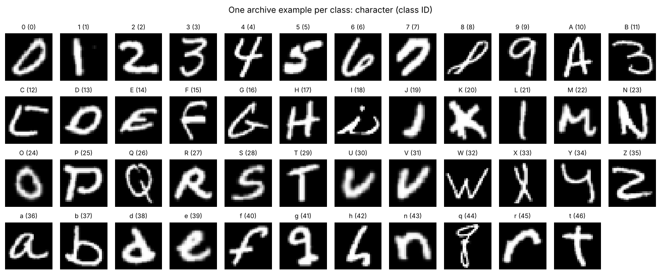
One archive example per class, labeled with its character and class ID. Compare the plot produced by your code with this reference image.
Task 01: Turn Images into Tensors and Batches
Task 01-1: Description (0 pts.)
From NumPy Arrays to Tensors
A PyTorch tensor is very much like a NumPy array: it has a shape, a data type (dtype), and supports @, broadcasting, slicing, and .sum(axis)-style reductions (PyTorch spells the argument dim). Tensors add two things we'll need: they can run on a GPU, and in HW07 they will be able to track gradients.
Before the network can use the images, we have to fix three things:
- The data type.
uint8arithmetic wraps around instead of producing large numbers. Weights and activations need fractional values, so we use 32-bit floats. - The scale. Dividing by
255puts every pixel in[0, 1]. Large, unscaled inputs make the outputs of the first layer large too, which (as we'll see in Task 02) makes a network harder to work with. - The shape. Image models in PyTorch expect
(batch, channels, height, width). Our grayscale images have one channel, so(9400, 28, 28)becomes(9400, 1, 28, 28). The FFN won't use the channel dimension, but HW07's CNN will, and keeping the standard layout means both models can share the same data.
Labels are different: they are class IDs, not measurements. A class ID of 12 is not "twice" class 6. PyTorch's loss functions expect class IDs as 64-bit integers (torch.long), so we keep them as integers.
Worked Example
pixels = np.array([[200, 100], [0, 255]], dtype=np.uint8)
pixels + pixels               # [[144, 200], [0, 254]]   <- 200 + 200 wrapped around!
t = torch.from_numpy(pixels.copy()).float() / 255.0
# tensor([[0.7843, 0.3922],
#         [0.0000, 1.0000]])
t.unsqueeze(0).shape          # torch.Size([1, 2, 2]): a new dimension of size 1 at position 0
Convert to float before dividing, and divide exactly once. Dividing twice silently produces images whose brightest pixel is 1/255, and every later result changes without an error message.
Your Task
Complete to_image_tensor(X):
- Input: a
uint8NumPy array with shape(n, 28, 28). - Return: a
torch.float32tensor with shape(n, 1, 28, 28)and values in[0, 1].
Then convert y_raw into a torch.long tensor named labels.
torch.from_numpy shares memory with the NumPy array. We call .copy() first so later changes to one can't silently change the other.
Python Help
a = np.zeros((3, 4), dtype=np.uint8)
torch.from_numpy(a.copy()).float().dtype   # torch.float32
torch.from_numpy(a.copy()).unsqueeze(1).shape   # torch.Size([3, 1, 4])
torch.from_numpy(np.array([3, 1])).long().dtype  # torch.int64 (also called torch.long)
Useful Links
Task 01-1: Code (0.25 pts.)
def to_image_tensor(X):
    # TODO: Convert to float, normalize to [0, 1] exactly once, and add a channel dimension.
    return None

# TODO: Keep the labels as integer class IDs.
labels = None
images = to_image_tensor(X_raw)

print('Images:', tuple(images.shape), images.dtype)
print('Pixel range:', float(images.min()), 'to', float(images.max()))
print('Labels:', tuple(labels.shape), labels.dtype)
Task 01-1: Expected Output (0 pts.)
Images: (9400, 1, 28, 28) torch.float32
Pixel range: 0.0 to 1.0
Labels: (9400,) torch.int64
Task 01-2: Description (0 pts.)
Splitting, Batching, and Flattening
Splitting. Just as in HW02–HW04, we need data the model never learns from. Remember that the file is grouped by class: if we simply took the first 940 rows for validation, the validation set would contain only five characters, and the training set would contain none of them. So we shuffle the row numbers once with a fixed seed and split the shuffled order. We randomly hold out 940 images (10%) for validation and keep 8,460 for training. The split uses a fixed seed so HW06 and HW07 see exactly the same examples. The test file stays closed until the very end of HW07: if we peeked at it while making decisions, it would stop being an honest estimate of performance on new evidence.
Batching. Neural networks are usually fed a minibatch of examples at a time rather than one example or the entire dataset. Two PyTorch tools handle this:
TensorDataset(images, labels)pairs each image with its label, sodataset[i]returns(image_i, label_i).DataLoader(dataset, batch_size=..., shuffle=...)walks through a dataset and returns one batch at a time. Each batch is a pair of tensors: images with shape(B, 1, 28, 28)and labels with shape(B,).
With shuffle=True, the loader visits the examples in a new random order on each pass. That matters for training in HW07. Shuffling changes the order of the examples, never which examples belong to the training or validation set. The last batch may be shorter than B: 940 validation images in batches of 128 give seven full batches and one batch of 44.
Flattening. A feed-forward network's first layer expects each example to be a single vector. We unroll each 28 × 28 image, row after row, into 784 numbers. The important detail is to flatten every dimension except the batch dimension:
Worked Example
batch = torch.arange(8.).reshape(2, 1, 2, 2)   # two tiny 2x2 "images"
batch.flatten().shape     # torch.Size([8])    <- both images merged into one vector!
batch.flatten(1).shape    # torch.Size([2, 4]) <- one row of 4 pixels per image
batch.flatten(1)
# tensor([[0., 1., 2., 3.],
#         [4., 5., 6., 7.]])
flatten(1) means "flatten starting at dimension 1", leaving dimension 0 (the batch) alone. Row i of the result still belongs to label i.
Notice what flattening throws away: the FFN no longer knows that pixel 0 and pixel 28 are vertical neighbors. It must learn any spatial relationships from data. HW07's CNN will keep that structure.
Your Task
The split and the make_loader helper are supplied.
- Create
train_loader(shuffled) andval_loader(not shuffled) withmake_loader. Use the default batch size of 128. - Take the first validation batch,
xb, yb = next(iter(val_loader)). (This line is supplied.) - Flatten
xbintoflat_batchwith shape(B, 784).
Python Help
loader = make_loader(some_dataset, shuffle=True)
for xb, yb in loader:     # one batch per loop iteration
    ...
xb, yb = next(iter(loader))   # just the first batch
Useful Links
Task 01-2: Code (0.5 pts.)
# Supplied: keep the same split across HW06 and HW07. Test data are opened only in HW07.
order = torch.randperm(len(images), generator=torch.Generator().manual_seed(42))
val_idx, train_idx = order[:940], order[940:]
train_data = TensorDataset(images[train_idx], labels[train_idx])
val_data = TensorDataset(images[val_idx], labels[val_idx])

def make_loader(data, shuffle=False, seed=42, batch_size=128):
    return DataLoader(data, batch_size=batch_size, shuffle=shuffle,
                      generator=torch.Generator().manual_seed(seed), num_workers=0)

# TODO: Build a shuffled training loader and an unshuffled validation loader.
train_loader = None
val_loader = None

xb, yb = next(iter(val_loader))

# TODO: Flatten every dimension except the batch dimension.
flat_batch = None

print('Train / validation:', len(train_data), '/', len(val_data))
print('Batches per pass: train', len(train_loader), '| validation', len(val_loader))
print('Last validation batch size:', len(val_data) % 128)
print('Image batch:', tuple(xb.shape), '| label batch:', tuple(yb.shape))
print('Flattened batch:', tuple(flat_batch.shape))
print('Row 0 is still image 0:', torch.equal(flat_batch[0], xb[0].reshape(-1)))
Task 01-2: Expected Output (0 pts.)
Train / validation: 8460 / 940
Batches per pass: train 67 | validation 8
Last validation batch size: 44
Image batch: (128, 1, 28, 28) | label batch: (128,)
Flattened batch: (128, 784)
Row 0 is still image 0: True
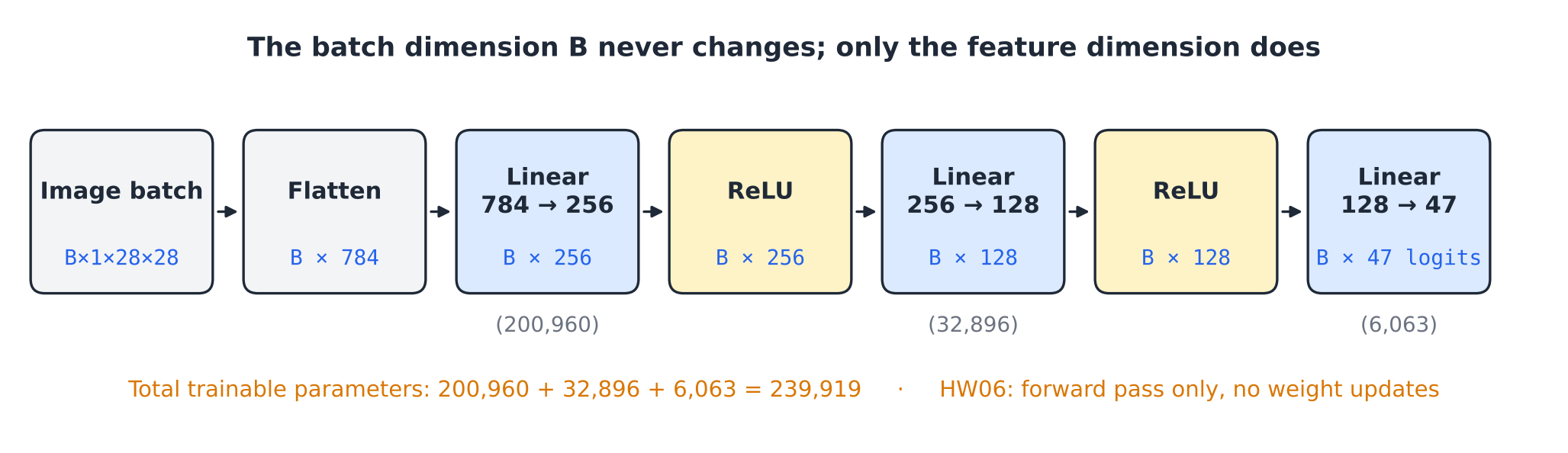
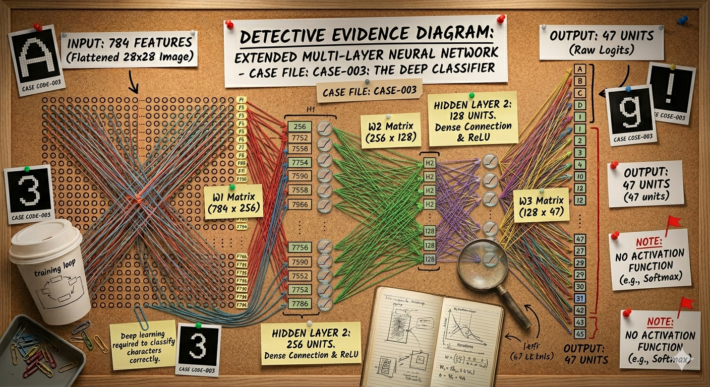
Figure 1. The network we will build this week. The batch dimension B stays separate through every layer; only the feature dimension changes. Numbers in parentheses are each layer's trainable parameters.
Task 02: Build an Affine Layer
Task 02-1: Description (0 pts.)
The Same Score, 256 Times at Once
In HW02 and HW03, one prediction was a weighted sum of the features plus a bias: $s = x\cdot w + b$. A linear layer (more precisely an affine layer, because of the bias) computes many of these weighted sums at once. Each output unit $j$ has its own weight vector $w_j$ and bias $b_j$:
$$h_j = x \cdot w_j + b_j .$$
Stack the weight vectors as the rows of a matrix $W$, and stack the examples as the rows of $X$. Then every output for every example comes from one matrix product:
$$Y = XW^{T} + b .$$
| Symbol | Meaning | Shape |
|---|---|---|
| $X$ | A batch of inputs, one example per row | (B, D) |
| $W$ | One row of weights per output unit | (H, D) |
| $b$ | One bias per output unit | (H,) |
| $Y$ | One row of outputs per example | (B, H) |
Here $D$ is the number of input features and $H$ the number of output units. We store $W$ as (H, D), "outputs by inputs", because that is also how PyTorch's nn.Linear stores it. That convention is why we multiply by $W^T$: (B, D) @ (D, H) gives (B, H).
The bias has shape (H,), but $XW^T$ has shape (B, H). Broadcasting adds the same bias row to every example, just as NumPy did in HW02.
Worked Example
Take $D=2$ inputs and $H=3$ output units:
$$W=\begin{bmatrix}1&2\\-1&1\\0&3\end{bmatrix},\qquad b=\begin{bmatrix}0&1&-1\end{bmatrix},\qquad x=\begin{bmatrix}1&2\end{bmatrix}.$$
Each output is the dot product of $x$ with one row of $W$, plus that unit's bias:
- Unit 0: $(1)(1) + (2)(2) + 0 = 5$
- Unit 1: $(1)(-1) + (2)(1) + 1 = 2$
- Unit 2: $(1)(0) + (2)(3) - 1 = 5$
So $y = [5, 2, 5]$. A second example $x=[3, 4]$ gives $[11, 2, 11]$. With both examples stacked as rows of $X$, one call to X @ W.T + b produces both rows.
Why Store the Input?
Our forward method also saves its input as self.X. Nothing uses it this week. In HW07, the gradient of the loss with respect to $W$ depends on the input that produced the output, so each layer must remember what it saw. Store it now and HW07's backward pass will slot into the same class.
Your Task
Complete LinearLayer.forward(X):
- Input:
Xwith shape(B, D). - Return:
X @ W.T + bwith shape(B, H). - Store the input in
self.Xbefore returning.
Use ordinary tensor operations: no nn.Linear and no automatic differentiation. The constructor is supplied for now; Task 02-2 explains its weight scale.
Python Help
A = torch.tensor([[1., 2.], [3., 4.]])   # (2, 2)
B = torch.tensor([[1., 0.], [0., 1.], [1., 1.]])   # (3, 2)
A @ B.T                                  # (2, 3): row i of A dotted with row j of B
A @ B.T + torch.tensor([10., 20., 30.])  # the bias is added to every row
Useful Links
nn.Lineardocumentation: note the shape of itsweight.
Task 02-1: Code (0.5 pts.)
class LinearLayer:
    def __init__(self, input_dim, output_dim, device='cpu'):
        self.W = torch.randn(output_dim, input_dim, device=device) * math.sqrt(2 / input_dim)
        self.b = torch.zeros(output_dim, device=device)

    def forward(self, X):
        # TODO: Cache the input for HW07, then apply the affine transformation.
        self.X = None
        return None

layer = LinearLayer(2, 3)
layer.W = torch.tensor([[1., 2.], [-1., 1.], [0., 3.]])
layer.b = torch.tensor([0., 1., -1.])
X_toy = torch.tensor([[1., 2.], [3., 4.]])

print(layer.forward(X_toy))
print('Output shape:', tuple(layer.forward(X_toy).shape))

first_layer = LinearLayer(784, 256)
print('First real layer:', tuple(flat_batch.shape), '->', tuple(first_layer.forward(flat_batch).shape))
Task 02-1: Expected Output (0 pts.)
tensor([[ 5.,  2.,  5.],
        [11.,  2., 11.]])
Output shape: (2, 3)
First real layer: (128, 784) -> (128, 256)
Task 02-2: Description (0 pts.)
Where Should the Weights Start?
In HW03 we started the perceptron's weights at zero. That will not work for a network with hidden layers. If every weight in a layer starts at the same value, every unit in that layer computes the same output for every example. In HW07, they would also receive the same update, so they would stay identical forever. A layer of 256 identical units is no better than one unit. Random starting weights break the symmetry.
How large should the random weights be? Each output of a linear layer adds up $D$ products. If the weights are too large, those sums grow layer after layer; if they're too small, they shrink toward zero. Either way, the last layer receives values that are huge or vanishingly small, and in HW07 the training updates will inherit the same problem.
Kaiming He and colleagues showed that for layers followed by ReLU, drawing weights from a normal distribution with variance $2/D$ keeps the typical size of the activations roughly steady from layer to layer:
$$W_{jk} \sim \mathcal{N}\!\left(0,\ \tfrac{2}{D}\right),\qquad b_j = 0 .$$
torch.randn draws standard normal values (variance 1); multiplying by $\sqrt{2/D}$ gives variance $2/D$. That is exactly what the supplied constructor does. The factor of 2 compensates for ReLU, which zeroes roughly half of its inputs.
Worked Example: How Big Does a Sum Get?
Suppose all $D=784$ inputs are about $0.5$ and the weights are random with standard deviation $\sigma$. A sum of $D$ independent random terms has a standard deviation about $\sqrt{D}$ times larger than one term:
- $\sigma = 1$: one output has standard deviation about $\sqrt{784}\times 0.5 = 14$.
- $\sigma = \sqrt{2/784} \approx 0.05$: about $\sqrt{784}\times 0.05\times 0.5 \approx 0.7$.
Stack three layers with $\sigma=1$ and the effect compounds: each layer multiplies the typical size again, by roughly a factor of 10 for our widths.
Your Task
- Complete the function
he_std(D): return the weight standard deviation thatLinearLayeruses for an input widthD. (Read it off the supplied constructor in Task 02-1.) - Run the supplied experiment. It pushes the real validation batch through three
ReLU(linear)layers of width 256 using three weight scales and prints the standard deviation of the activations after each layer. It also builds a layer whose weights are all zero and checks whether its four units produce different outputs.
Compare the three rows, then answer Task 02-3.
Useful Links
Task 02-2: Code (0.25 pts.)
def he_std(D):
    # TODO: Return the weight standard deviation LinearLayer uses for an input width D.
    return None

# Supplied: the weight standard deviation for each of the three starting rules.
def weight_std(rule, D):
    if rule == 'too small (0.01)':
        return 0.01
    if rule == 'too large (1.0)':
        return 1.0
    return he_std(D)

def activation_scales(X, rule, widths=(256, 256, 256), seed=0):
    generator = torch.Generator().manual_seed(seed)
    stds, H = [], X
    for width in widths:
        W = torch.randn(width, H.shape[1], generator=generator) * weight_std(rule, H.shape[1])
        H = (H @ W.T).clamp_min(0)
        stds.append(round(float(H.std()), 3))
    return stds

for rule in ['too small (0.01)', 'He: sqrt(2 / D)', 'too large (1.0)']:
    print(f'{rule:>17}: activation std after layers 1, 2, 3 = {activation_scales(flat_batch, rule)}')

zero_layer = LinearLayer(784, 4)
zero_layer.W = torch.zeros(4, 784)
print('Zero-initialized units produce identical outputs:',
      bool((zero_layer.forward(flat_batch) == zero_layer.forward(flat_batch)[:, :1]).all()))
Task 02-2: Reference Output (0 pts.)
 too small (0.01): activation std after layers 1, 2, 3 = [0.061, 0.006, 0.001]
  He: sqrt(2 / D): activation std after layers 1, 2, 3 = [0.308, 0.277, 0.25]
  too large (1.0): activation std after layers 1, 2, 3 = [6.09, 61.951, 633.286]
Zero-initialized units produce identical outputs: True
Task 02-3: Written Response (0.125 pts.)
- Using your printed standard deviations, describe what happens to the activations as they pass through three layers with each weight scale. Why might the "too large" row cause trouble for the final scores, and why might the "too small" row?
[ANSWER]
- The HW03 perceptron started at zero weights and learned perfectly well. Why does a zero start fail for a layer with 256 hidden units?
[ANSWER]
Task 03: Add a Nonlinearity
Task 03-1: Description (0 pts.)
Why Can't We Just Stack Linear Layers?
It's tempting to think that stacking more linear layers makes a more powerful model. It doesn't. Two linear layers in a row are still just one linear layer:
$$\big(XW_1^T + b_1\big)W_2^T + b_2 \;=\; X\underbrace{(W_2W_1)^T}_{\text{one matrix}} + \underbrace{\big(b_1W_2^T + b_2\big)}_{\text{one bias}} .$$
No matter how many we stack, the result can only draw the same kind of straight (hyperplane) boundary as HW03's logistic regression. HW04 handled curved boundaries by swapping in an RBF kernel. Neural networks take a different route: they insert a nonlinear activation function between the linear layers, so the composition can no longer be multiplied out into one matrix.
ReLU
The rectified linear unit keeps positive values and replaces negative values with zero, independently for each entry:
$$\operatorname{ReLU}(z)=\max(0, z).$$
It is cheap to compute, and (as you'll see in HW07) its derivative is simply 1 for positive inputs and 0 for negative ones. Each hidden unit becomes a little "detector" that is either silent or responds in proportion to how strongly its pattern is present.
Worked Example
z = torch.tensor([[-2.0, 0.0, 3.0],
                  [ 1.5, -0.1, -7.0]])
z.clamp_min(0)
# tensor([[0.0, 0.0, 3.0],
#         [1.5, 0.0, 0.0]])
The shape never changes: ReLU acts on each entry separately. Like LinearLayer, our ReLU stores its input. In HW07, the backward pass needs to know which entries were positive.
Your Task
Complete ReLU.forward(X):
- Store the input in
self.X. - Return a tensor of the same shape, with negative entries replaced by zero.
The supplied code then checks the algebra above. It builds two small random linear layers, merges them into one layer, and compares the outputs with and without a ReLU in between.
Python Help
torch.tensor([-1., 2.]).clamp_min(0)          # tensor([0., 2.])
torch.maximum(torch.tensor([-1., 2.]), torch.tensor(0.))   # same result
torch.allclose(a, b, atol=1e-6)               # True when every entry is (nearly) equal
Task 03-1: Code (0.25 pts.)
class ReLU:
    def forward(self, X):
        # TODO: Cache the input for HW07, then keep only its positive values.
        self.X = None
        return None

print(ReLU().forward(torch.tensor([[-2.0, 0.0, 3.0], [1.5, -0.1, -7.0]])))

# Supplied: two stacked linear layers versus one merged layer.
torch.manual_seed(0)
first, second = LinearLayer(4, 5), LinearLayer(5, 3)
first.b, second.b = torch.randn(5), torch.randn(3)
merged = LinearLayer(4, 3)
merged.W = second.W @ first.W
merged.b = first.b @ second.W.T + second.b
X_small = torch.randn(6, 4)

stacked = second.forward(first.forward(X_small))
with_relu = second.forward(ReLU().forward(first.forward(X_small)))
print('Two linear layers equal one merged layer:', torch.allclose(stacked, merged.forward(X_small), atol=1e-5))
print('With ReLU in between, still equal:      ', torch.allclose(with_relu, merged.forward(X_small), atol=1e-5))
Task 03-1: Expected Output (0 pts.)
tensor([[0.0000, 0.0000, 3.0000],
        [1.5000, 0.0000, 0.0000]])
Two linear layers equal one merged layer: True
With ReLU in between, still equal:       False
Task 03-2: Written Response (0.125 pts.)
Our network will be Linear → ReLU → Linear → ReLU → Linear. Why is there no ReLU after the final layer? (Hint: think about what a negative final score should be allowed to mean for one of the 47 characters.) In one sentence, compare the role of ReLU here with the role of the RBF kernel in HW04.
[ANSWER]
Story Progression
The intern has been watching over your shoulder. "So it's just multiplying and adding, then throwing away the negatives? I could do that with a calculator." Caulfield points out that a single image needs about 240,000 multiplications. The intern goes to find a bigger calculator.
The network can now produce 47 numbers for each image. Before we assemble it, we need to decide what those numbers mean and how to measure whether they're any good.
Task 04: Turn Logits into a Stable Loss
Task 04-1: Description (0 pts.)
From Scores to Probabilities
The final layer produces one unrestricted real number per class, called a logit. Larger means "more likely this class", but logits are not probabilities: they can be negative, and they don't add up to one.
In HW03, logistic regression turned one score $s$ into a probability with the sigmoid, $\sigma(s)=\frac{1}{1+e^{-s}}$. With 47 classes we need 47 probabilities that sum to one. The softmax function does this:
$$p_j=\frac{e^{z_j}}{\sum_{k} e^{z_k}} .$$
Exponentiating makes every value positive; dividing by the total makes them sum to one. A logit that is 1 larger than another gets $e \approx 2.7$ times the probability.
Softmax generalizes the sigmoid. With two classes and logits $[s, 0]$:
$$p_0=\frac{e^{s}}{e^{s}+e^{0}}=\frac{1}{1+e^{-s}}=\sigma(s).$$
So HW03's logistic regression is exactly a one-layer network with two output classes.
Worked Example
For logits $z=[2, 1, 0]$:
| Class 0 | Class 1 | Class 2 | Total | |
|---|---|---|---|---|
| $z_j$ | 2 | 1 | 0 | |
| $e^{z_j}$ | 7.389 | 2.718 | 1.000 | 11.107 |
| $p_j$ | 0.665 | 0.245 | 0.090 | 1.000 |
The Overflow Problem
A 32-bit float can't represent numbers larger than about $3.4\times10^{38}$, and $e^{89}$ already exceeds that. A logit of 1000 is unusual but entirely possible early in training:
torch.exp(torch.tensor([1000., 1001., 999.]))   # tensor([inf, inf, inf])
# inf / inf = nan, and one nan contaminates every later calculation.
The fix uses a property of softmax: adding the same constant to every logit doesn't change the probabilities, because $e^{c}$ cancels from the numerator and the denominator. If we subtract the largest logit first, the largest exponent becomes $e^0 = 1$ and nothing can overflow:
$$[1000,1001,999] - 1001 = [-1, 0, -2]\ \Rightarrow\ p = [0.245,\ 0.665,\ 0.090].$$
Working in Log Space
The loss in Task 04-2 needs $\log p_j$, not $p_j$. Taking the log of the softmax gives
$$\log p_j = z_j - \log\sum_k e^{z_k} .$$
The second term is called log-sum-exp. Computing $\log p$ this way, with the max subtracted first, never forms a tiny probability only to take its log. For $[2,1,0]$: $\log(11.107)=2.408$, so $\log p = [-0.408, -1.408, -2.408]$.
Your Task
Complete log_softmax(logits) for a (B, C) tensor of logits, one row per example:
- Subtract each row's maximum logit from that row (use
keepdim=Trueso the shapes broadcast). - Compute each row's log-sum-exp of the shifted logits: exponentiate, sum across classes, take the log. Do not call
torch.logsumexportorch.log_softmax; the point is to see how the stable version works. - Return the shifted logits minus that row's log-sum-exp.
The supplied code compares your result with PyTorch's F.log_softmax, including on logits large enough to overflow a naive softmax.
Python Help
Z = torch.tensor([[2., 1., 0.], [5., 7., 6.]])
Z.max(dim=1, keepdim=True).values   # tensor([[2.], [7.]]): shape (2, 1), one max per row
Z.exp().sum(dim=1, keepdim=True)    # one total per row, shape (2, 1)
Useful Links
Task 04-1: Code (0.5 pts.)
def log_softmax(logits):
    # TODO: Subtract each row's maximum logit.
    shifted = None
    # TODO: Subtract each row's log-sum-exp from the shifted logits.
    return None

small = torch.tensor([[2., 1., 0.]])
huge = torch.tensor([[1000., 1001., 999.]])
print('Naive softmax of huge logits:', torch.exp(huge) / torch.exp(huge).sum())
print('Log probabilities of [2, 1, 0]:', log_softmax(small).numpy().round(3))
print('Probabilities of [2, 1, 0]:', log_softmax(small).exp().numpy().round(3))
print('Probabilities of [1000, 1001, 999]:', log_softmax(huge).exp().numpy().round(3))

random_logits = torch.randn(5, 47) * 30
print('Each row sums to one:', torch.allclose(log_softmax(random_logits).exp().sum(dim=1), torch.ones(5)))
print('Matches F.log_softmax:', torch.allclose(log_softmax(random_logits), F.log_softmax(random_logits, dim=1), atol=1e-5))

two_class = log_softmax(torch.tensor([[1.5, 0.]])).exp()[0, 0]
print(f'Two-class softmax {float(two_class):.4f} vs sigmoid {float(torch.sigmoid(torch.tensor(1.5))):.4f}')
Task 04-1: Expected Output (0 pts.)
Naive softmax of huge logits: tensor([[nan, nan, nan]])
Log probabilities of [2, 1, 0]: [[-0.408 -1.408 -2.408]]
Probabilities of [2, 1, 0]: [[0.665 0.245 0.09 ]]
Probabilities of [1000, 1001, 999]: [[0.245 0.665 0.09 ]]
Each row sums to one: True
Matches F.log_softmax: True
Two-class softmax 0.8176 vs sigmoid 0.8176
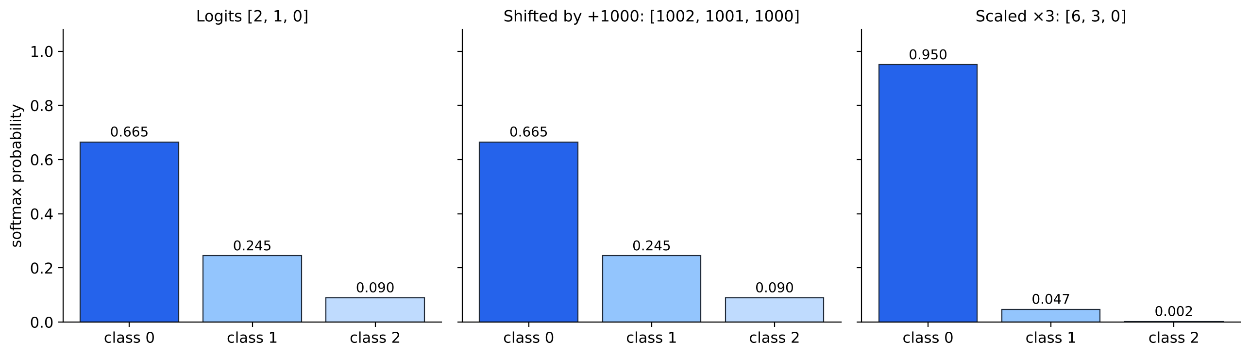
Figure 2. Softmax turns logits into probabilities. Shifting every logit by the same amount (middle) leaves the probabilities unchanged; multiplying them by a constant (right) makes the prediction more or less confident.
Task 04-2: Description (0 pts.)
How Wrong Was That Prediction?
In HW03 we measured a probability's quality with the log loss: $-\log p$ of the outcome that actually happened. Cross-entropy is the same idea for many classes. For one example whose true class is $y$,
$$\ell = -\log p_{y} = -\big(z_y - \log\textstyle\sum_k e^{z_k}\big).$$
Only the probability assigned to the correct class matters. If the model gives the true class probability 1, the loss is 0. As that probability falls toward 0, the loss grows without bound: a confident wrong answer is punished heavily. For a batch, we report the mean loss over the $B$ examples:
$$L = \frac{1}{B}\sum_{i=1}^{B} -\log p_{i,\,y_i} .$$
With two classes, this is exactly HW03's log loss.
Worked Example
Using the log probabilities from Task 04-1 for logits $[2,1,0]$:
- If the true class is 0: $\ell = -(-0.408) = 0.408$. The model's favorite is correct.
- If the true class is 2: $\ell = -(-2.408) = 2.408$. The correct class got only 9% probability.
For a batch containing both examples, $L = (0.408 + 2.408)/2 = 1.408$.
Selecting One Entry per Row
log_softmax(logits) has shape (B, C). We need entry [i, y_i] from each row i. Paired integer indexing does that in one step: index with a tensor of row numbers and a tensor of column numbers of the same length.
log_p = torch.tensor([[-0.4, -1.4, -2.4],
                      [-0.4, -1.4, -2.4]])
targets = torch.tensor([0, 2])
log_p[torch.arange(2), targets]   # tensor([-0.4, -2.4]): entries [0, 0] and [1, 2]
Note that log_p[:, targets] is not the same thing: it returns a (2, 2) table containing columns 0 and 2 for every row.
A Word on PyTorch's Version
F.cross_entropy(logits, targets) does all of this internally: it takes raw logits, applies the stable log-softmax, and selects the correct classes. A very common bug is to apply softmax first and pass probabilities to F.cross_entropy. That applies softmax twice and quietly computes the wrong loss. Always give it logits.
Your Task
Complete cross_entropy(logits, targets):
- Input:
logitswith shape(B, C)andtargetswith shape(B,)containing integer class IDs. - Return: a scalar tensor: the mean negative log probability of each example's correct class.
Use your log_softmax. The supplied code compares your loss with F.cross_entropy on the worked example and on the huge logits from Task 04-1.
Useful Links
Task 04-2: Code (0.5 pts.)
def cross_entropy(logits, targets):
    # TODO: Select each example's correct-class log probability and average the negatives.
    log_p = None
    return None

pair = torch.tensor([[2., 1., 0.], [2., 1., 0.]])
pair_targets = torch.tensor([0, 2])
print(f'Worked example loss: ours {float(cross_entropy(pair, pair_targets)):.4f} | '
      f'PyTorch {float(F.cross_entropy(pair, pair_targets)):.4f}')

huge_pair = torch.tensor([[1000., 1001., 999.], [-1000., -1001., -999.]])
huge_targets = torch.tensor([1, 2])
print(f'Huge logits loss:    ours {float(cross_entropy(huge_pair, huge_targets)):.4f} | '
      f'PyTorch {float(F.cross_entropy(huge_pair, huge_targets)):.4f}')

probabilities = F.softmax(pair, dim=1)
print(f'Common bug, softmax passed to F.cross_entropy: {float(F.cross_entropy(probabilities, pair_targets)):.4f}')

uniform = torch.zeros(4, 47)   # every class gets the same logit
print(f'Loss when all 47 classes are equally likely: {float(cross_entropy(uniform, torch.tensor([0, 5, 20, 46]))):.4f}')
Task 04-2: Expected Output (0 pts.)
Worked example loss: ours 1.4076 | PyTorch 1.4076
Huge logits loss:    ours 0.4076 | PyTorch 0.4076
Common bug, softmax passed to F.cross_entropy: 1.0848
Loss when all 47 classes are equally likely: 3.8501
Task 04-3: Written Response (0.125 pts.)
The last printed line is the loss of a model that assigns every class the same probability. Show where the number 3.8501 comes from. In HW07, a training loss that stays near this value after many updates tells us something specific about the model. What?
[ANSWER]
Task 05: Assemble the Network
Task 05-1: Description (0 pts.)
Putting the Pieces in Order
Our feed-forward network (also called a multilayer perceptron) is
$$\texttt{784}\xrightarrow{\text{Linear}}\texttt{256}\xrightarrow{\text{ReLU}}\texttt{256}\xrightarrow{\text{Linear}}\texttt{128}\xrightarrow{\text{ReLU}}\texttt{128}\xrightarrow{\text{Linear}}\texttt{47 logits}.$$
The two middle widths (256 and 128) are hyperparameters: design choices, like k in HW01 or C in HW04. The first and last widths are not choices: 784 is the number of pixels and 47 the number of classes. As Task 03-2 discussed, the last layer has no ReLU.
The forward pass is just function composition: flatten the batch, then feed each layer's output into the next. Every example's row stays independent of the other rows, so a batch of 4 and a batch of 128 use exactly the same code.
Worked Example: Counting Parameters
Each linear layer has one weight per (output, input) pair plus one bias per output: $H\times D + H$. ReLU has nothing to learn.
| Layer | Weights | Biases | Parameters |
|---|---|---|---|
| Linear 784 → 256 | 784 × 256 = 200,704 | 256 | 200,960 |
| Linear 256 → 128 | 256 × 128 = 32,768 | 128 | 32,896 |
| Linear 128 → 47 | 128 × 47 = 6,016 | 47 | 6,063 |
| Total | 239,919 |
Almost 84% of the parameters are in the first layer: one weight for every pixel for every one of the 256 units. Training will adjust all 239,919 numbers. For comparison, HW04's SVM learned 7 (six feature weights and a bias, for the linear kernel).
Your Task
Complete ScratchFFN.forward(X):
- Input: an image batch with shape
(B, 1, 28, 28). - Return: logits with shape
(B, 47).
- Flatten everything except the batch dimension.
- Pass the result through each layer in
self.layers, in order, calling each layer'sforward.
The supplied code traces the shape after every layer, counts the parameters, and evaluates the loss of the untrained network on one batch.
Python Help
toy_layers = [LinearLayer(2, 3), ReLU(), LinearLayer(3, 1)]
H = torch.ones(5, 2)            # 5 examples, 2 features each
for layer in toy_layers:
    H = layer.forward(H)        # each layer's output becomes the next layer's input
print(H.shape)                  # torch.Size([5, 1])
Task 05-1: Code (0.5 pts.)
class ScratchFFN:
    def __init__(self, device='cpu'):
        self.layers = [LinearLayer(784, 256, device), ReLU(),
                       LinearLayer(256, 128, device), ReLU(),
                       LinearLayer(128, 47, device)]

    def forward(self, X):
        # TODO: Flatten each image, then apply every layer in order.
        return None

torch.manual_seed(42)
model = ScratchFFN()
xb4, yb4 = next(iter(make_loader(val_data, batch_size=4)))

activations = xb4.flatten(1)
shapes = [tuple(activations.shape)]
for layer in model.layers:
    activations = layer.forward(activations)
    shapes.append((type(layer).__name__, tuple(activations.shape)))
print('Input:', shapes[0])
for name, shape in shapes[1:]:
    print(f'  after {name:<11} {shape}')

parameter_count = sum(layer.W.numel() + layer.b.numel() for layer in model.layers if hasattr(layer, 'W'))
print('Trainable parameters:', parameter_count)
print('forward() output shape:', tuple(model.forward(xb4).shape))
print(f'Untrained loss on the first validation batch: {float(cross_entropy(model.forward(xb), yb)):.4f}')
Task 05-1: Expected Output (0 pts.)
The architecture lines are exact. The loss depends on the random starting weights; yours should match when you run the cells in order.
Input: (4, 784)
  after LinearLayer (4, 256)
  after ReLU        (4, 256)
  after LinearLayer (4, 128)
  after ReLU        (4, 128)
  after LinearLayer (4, 47)
Trainable parameters: 239919
forward() output shape: (4, 47)
Untrained loss on the first validation batch: 3.9775
Story Progression
The network is assembled: 239,919 numbers, every one of them chosen at random. Caulfield wants to know whether it works. The honest answer is that we don't know yet whether it computes what we think it computes, never mind whether it reads handwriting.
Those are two different questions, and the next task separates them. First we'll check our scratch implementation against PyTorch's. Then we'll see what an untrained network actually predicts.
Task 06: Check Against PyTorch and Inspect the Predictions
Task 06-1: Description (0 pts.)
The Same Network, Written the Library Way
In practice, nobody writes LinearLayer by hand. PyTorch provides the same building blocks:
| Our scratch version | PyTorch version | Notes |
|---|---|---|
X.flatten(1) |
nn.Flatten() |
Flattens from dimension 1 by default, keeping the batch |
LinearLayer(D, H) |
nn.Linear(D, H) |
.weight has shape (H, D) and .bias shape (H,), exactly like our W and b |
ReLU() |
nn.ReLU() |
|
| list of layers + loop | nn.Sequential(...) |
Calls each module in order |
cross_entropy |
F.cross_entropy |
Takes raw logits |
A PyTorch model is a class that inherits from nn.Module, creates its layers in __init__, and defines forward. You call the model like a function, reference(xb), and PyTorch calls forward for you.
Same Architecture Is Not the Same Function
nn.Linear draws its own random starting weights, using a different rule than ours. So two networks with identical architecture will produce different logits until they also have identical parameters. To test our implementation, we copy every weight and bias from the scratch model into the PyTorch model, then feed both the same images. If the logits agree (to within floating-point rounding), our forward pass computes the same function as PyTorch's.
When copying, wrap the code in torch.no_grad(). PyTorch parameters normally track every operation for HW07's automatic differentiation; an in-place copy into them is only allowed when that tracking is turned off.
Your Task
- Complete
TorchFFN.__init__: buildself.layerswithnn.Sequential, matching the scratch architecture exactly:Flatten, threeLinearlayers, and aReLUafter each of the first two. - Complete
copy_to_torch(scratch, reference). The supplied code pairs the scratch linear layers with the PyTorch linear layers in order. For each pair, copyWinto.weightandbinto.biaswith.copy_().
The supplied code prints the largest difference between the two models' logits.
Python Help
net = nn.Sequential(nn.Linear(3, 2), nn.ReLU())
net[0].weight.shape                 # torch.Size([2, 3])
with torch.no_grad():
    net[0].weight.copy_(torch.ones(2, 3))   # overwrite in place
Useful Links
Task 06-1: Code (0.5 pts.)
class TorchFFN(nn.Module):
    def __init__(self):
        super().__init__()
        # TODO: Match the scratch architecture exactly.
        self.layers = None

    def forward(self, X):
        return self.layers(X)

def copy_to_torch(scratch, reference):
    scratch_linear = [layer for layer in scratch.layers if isinstance(layer, LinearLayer)]
    torch_linear = [layer for layer in reference.layers if isinstance(layer, nn.Linear)]
    with torch.no_grad():
        for ours, theirs in zip(scratch_linear, torch_linear):
            # TODO: Copy this layer's weights and bias into the PyTorch layer.
            pass

reference = TorchFFN()
print(reference)

with torch.no_grad():
    before = (model.forward(xb) - reference(xb)).abs().max()
    copy_to_torch(model, reference)
    after = (model.forward(xb) - reference(xb)).abs().max()
print(f'Largest logit difference before copying weights: {float(before):.2f}')
print('Largest logit difference after copying is below 1e-5:', bool(after < 1e-5))
Task 06-1: Expected Output (0 pts.)
The difference before copying depends on PyTorch's random initialization and will vary; it should be well above zero. The other lines are exact.
TorchFFN(
  (layers): Sequential(
    (0): Flatten(start_dim=1, end_dim=-1)
    (1): Linear(in_features=784, out_features=256, bias=True)
    (2): ReLU()
    (3): Linear(in_features=256, out_features=128, bias=True)
    (4): ReLU()
    (5): Linear(in_features=128, out_features=47, bias=True)
  )
)
Largest logit difference before copying weights: 2.04
Largest logit difference after copying is below 1e-5: True
Task 06-2: Description (0 pts.)
What Does an Untrained Network Predict?
Our two implementations agree. That tells us the calculation is right. It tells us nothing about whether the predictions are any good, because neither model has learned anything.
To measure that, we evaluate the model on the whole validation set. An evaluation function has to be careful about one detail: the last batch is shorter. Averaging eight per-batch mean losses would give the 44-example batch the same weight as each 128-example batch. Instead, add up the total loss and the number correct over every batch, and divide by the total number of examples once at the end:
$$\text{accuracy}=\frac{\sum_{\text{batches}}\#\text{correct}}{\sum_{\text{batches}}B},\qquad \text{loss}=\frac{\sum_{\text{batches}}\sum_{i}\ell_i}{\sum_{\text{batches}}B}.$$
F.cross_entropy(..., reduction='sum') returns the batch total instead of the mean. The predicted class is the one with the largest logit, logits.argmax(dim=1). We don't need softmax for this: softmax never changes which entry is largest.
Worked Example
Two batches: 3 of 4 correct with total loss 2.0, then 0 of 1 correct with loss 4.0.
- Correct: accuracy $= (3+0)/(4+1) = 0.60$; loss $= (2.0+4.0)/5 = 1.2$.
- Averaging the batch accuracies instead: $(0.75 + 0)/2 = 0.375$. That gives the one-example batch the same weight as the four-example batch.
What Should We Expect?
Guessing uniformly among 47 classes is right about $1/47 \approx 2.1\%$ of the time, with loss $\log 47 \approx 3.85$ (Task 04-3). A particular random network won't hit those numbers exactly. It might favor a few classes for most images, or be slightly more confident than uniform guessing. Its predicted "confidence" (the largest softmax probability) should still be low, because nothing in its weights has been fitted to handwriting.
Your Task
Complete the loop inside evaluate(model, loader) so it accumulates total_loss, correct, and count across batches. It works for both the scratch model and the PyTorch model.
Python Help
logits = torch.tensor([[0.1, 2.0], [3.0, -1.0], [0.0, 0.5]])
targets = torch.tensor([1, 1, 1])
logits.argmax(dim=1)                                  # tensor([1, 0, 1])
int((logits.argmax(dim=1) == targets).sum())          # 2 correct
float(F.cross_entropy(logits, targets, reduction='sum'))   # total, not mean
Task 06-2: Code (0.25 pts.)
@torch.no_grad()
def evaluate(model, loader):
    total_loss, correct, count = 0., 0, 0
    for xb_eval, yb_eval in loader:
        logits = model(xb_eval) if isinstance(model, nn.Module) else model.forward(xb_eval)
        # TODO: Accumulate the summed loss, number correct, and number of examples.
        total_loss += 0
        correct += 0
        count += 0
    return {'loss': round(total_loss / count, 4), 'accuracy': round(correct / count, 4)}

print('Untrained scratch FFN, validation:', evaluate(model, val_loader))
print('Untrained PyTorch FFN, validation:', evaluate(reference, val_loader))
print(f'Uniform guessing: loss {math.log(47):.4f}, accuracy {1 / 47:.4f}')

with torch.no_grad():
    probabilities = log_softmax(model.forward(xb)).exp()
    confidence, predicted = probabilities.max(dim=1)
print(f'Average confidence in its own prediction: {float(confidence.mean()):.3f}')
print('Distinct classes predicted for 128 images:', len(predicted.unique()))

# Supplied: show the first 12 validation images with the untrained model's guesses.
show_characters(xb[:12, 0].numpy(),
                [f'true {classes[int(t)]}\nguess {classes[int(p)]} ({float(c):.2f})'
                 for t, p, c in zip(yb[:12], predicted[:12], confidence[:12])],
                columns=6, suptitle='The untrained network\'s guesses (and confidence)')
Task 06-2: Reference Output (0 pts.)
Your numbers should match when you run the cells in order. Small floating-point differences across machines are normal.
Untrained scratch FFN, validation: {'loss': 3.9704, 'accuracy': 0.0234}
Untrained PyTorch FFN, validation: {'loss': 3.9704, 'accuracy': 0.0234}
Uniform guessing: loss 3.8501, accuracy 0.0213
Average confidence in its own prediction: 0.056
Distinct classes predicted for 128 images: 17
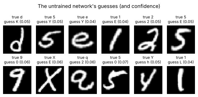
The untrained network's guesses and confidence on the first 12 validation images.
Task 07: Report the Results to Caulfield
Task 07-1: Written Response (0.375 pts.)
- Our scratch network and PyTorch's network agreed to within $10^{-5}$, yet both get only a few percent of the validation set right. Explain why both statements can be true. What did the comparison verify, and what did it not verify?
[ANSWER]
- Report the untrained validation loss and accuracy. Compare them with uniform guessing ($\log 47$ and $1/47$). Why isn't a random network exactly at chance?
[ANSWER]
- Before computing the loss, we keep the network's output as logits rather than converting it to probabilities. Give two reasons, using what you saw in Task 04.
[ANSWER]
Story Progression
Your report goes to Caulfield: the network computes exactly what it's supposed to, and it reads handwriting about as well as a person picking characters out of a hat. The intern feels much better about his own accuracy.
Caulfield isn't discouraged. A calculation we can trust is the foundation; what's missing is learning. Every one of those 239,919 weights needs to be nudged, a little at a time, in the direction that lowers the loss you just implemented. That requires knowing how the loss changes when each weight changes.
In HW07, we'll implement the backward pass, train the network on the archive, compare it with PyTorch's trained version and a convolutional network, and finally point it at the recovered letters.

Task 08: Export the Completed Notebook (0 pts.)
- Complete your code and written responses, and run the cells above in order. Compare your results with the expected and reference outputs.
- Save your notebook, including its outputs. Set
GENERATE = Truebelow when you are ready to export. - In Colab, the cell captures the current notebook and its outputs. Locally, it reads the saved notebook at
NOTEBOOK_PATH; adjust that path if you saved your copy elsewhere. - Download
homework06.htmland open it in a browser. Check that your name, NETID, code, written answers, and outputs appear.
Submit only homework06.html on Canvas. The exporter does not rerun your code.
Task 08-1: Code (0 pts.)
GENERATE = False
NOTEBOOK_PATH = DATA_ROOT / 'homeworks' / 'homework06' / 'homework06.ipynb'

if GENERATE:
    import json
    import nbformat
    from nbconvert import HTMLExporter
    from pathlib import Path

    try:
        from google.colab import _message, files
    except ImportError:
        current = nbformat.read(NOTEBOOK_PATH, as_version=4)
        html_path = NOTEBOOK_PATH.with_name('homework06.html')
        in_colab = False
    else:
        captured = _message.blocking_request('get_ipynb', timeout_sec=10)
        current = nbformat.reads(json.dumps(captured['ipynb']), as_version=4)
        html_path = Path('/content/homework06.html')
        in_colab = True

    exporter = HTMLExporter()
    exporter.embed_images = True
    report_html, _ = exporter.from_notebook_node(current)
    html_path.write_text(report_html, encoding='utf-8')
    print(f'Exported {html_path.name}. Open it in a browser before submitting.')

    if in_colab:
        files.download(str(html_path))
    else:
        print(f'Saved to: {html_path}')
else:
    print('Export disabled. Set GENERATE = True when ready.')
Task 08-1: Expected Output (0 pts.)
Export disabled. Set GENERATE = True when ready.