CSE 30124 - Introduction to Artificial Intelligence: Lab 03 (5 pts.)

• NETID:

This assignment covers the following topics:

• Creating and manipulating PyTorch tensors
• Converting between NumPy arrays and PyTorch tensors
• Defining models with nn.Module
• Loading data with Dataset and DataLoader
• The PyTorch training loop (zero_grad, backward, step)
• Building multi-layer feed-forward networks

It will consist of 8 tasks:

Task ID	Description	Points
00	Setup	0
01	NumPy ↔ Tensor Conversion	1
02	Define a Single-Layer Classifier	0.5
03	Create a DataLoader	1
04	Train the Single-Layer Model	0.5
05	Build a Multi-Layer FFN	1
06	Train and Compare	1
07	Generate Police Report	0

Please complete all sections. Some questions will require written answers, while others will involve coding. Be sure to run your code cells to verify your solutions.

Story Progression

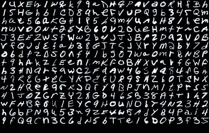
Your image segmentation work paid off — the forensics team now has individual letter images extracted from the ransom notes. But identifying what character each letter actually is? That's a job for a neural network.

Evidence 1: Letters extracted from the ransom note — but what do they say?

You know that if you're going to try and convert these letter images to an ascii character (which you could structure as a supervised classification task), you'll need some training data. Luckily, the police have kept records from past kidnapping cases for you and have created a dataset of the letter clippings used in those cases and what they actually were. They call the dataset EMNIST, which is available on their evidence servers.

Evidence 2: Examples from the EMNIST dataset the police have.

Director Bryant tells you the department has a character recognition system, but it runs on PyTorch — a deep learning framework you haven't used before. Before you can feed the evidence through the classifier, you need to learn how PyTorch represents and processes data. Detective Gaff slides a PyTorch tutorial across the table. "Better start reading," he says.

Task 00: Setup (0 pts.)

Task 00: Code (0 pts.)

import os
import numpy as np
import matplotlib.pyplot as plt

try:
    import google.colab
    REPO_URL = "https://github.com/wtheisen/nd-cse-30124-homeworks.git"
    REPO_NAME = "nd-cse-30124-homeworks"
    LAB_FOLDER = "evidence/lab03"

    %cd /content/
    if not os.path.exists(REPO_NAME):
        !git clone {REPO_URL}

    %cd {REPO_NAME}/{LAB_FOLDER}

except ImportError:
    print("Not running on Colab - assuming local setup.")

import torch
import torch.nn as nn
import torch.nn.functional as F
from torch.utils.data import TensorDataset, DataLoader

print(f"PyTorch version: {torch.__version__}")
print(f"NumPy version:   {np.__version__}")

# Device selection (GPU if available, otherwise CPU)
device = torch.device('cuda' if torch.cuda.is_available() else 'mps' if torch.backends.mps.is_available() else 'cpu')
print(f"Using device:    {device}")
print("Setup complete!")

/content
Cloning into 'nd-cse-30124-homeworks'...
remote: Enumerating objects: 721, done.
remote: Counting objects: 100% (137/137), done.
remote: Compressing objects: 100% (33/33), done.
remote: Total 721 (delta 127), reused 104 (delta 104), pack-reused 584 (from 1)
Receiving objects: 100% (721/721), 229.02 MiB | 29.01 MiB/s, done.
Resolving deltas: 100% (269/269), done.
Updating files: 100% (315/315), done.
/content/nd-cse-30124-homeworks/evidence/lab03
PyTorch version: 2.10.0+cpu
NumPy version:   2.0.2
Using device:    cpu
Setup complete!

Task 01: NumPy ↔ Tensor Conversion (1 pt.)

The EMNIST dataset used by the forensics classifier is stored as NumPy .npz files. Load the training data, convert the images and labels to PyTorch tensors, and verify the conversion.

Steps:

1. Load the .npz file with np.load()
2. Extract the X (images) and y (labels) arrays
3. Flatten images from (n, 28, 28) to (n, 784) and normalize pixel values to [0, 1]
4. Convert images to a float32 tensor and labels to a long tensor (required by PyTorch's loss functions)
5. Print shapes, dtypes, and pixel value range

Useful functions:

• np.load("path.npz") — returns a dict-like object; access arrays with data['X'], data['y']
• array.reshape(-1, 784) — flattens each 28×28 image to a 784-length vector (-1 means "infer this dimension")
• torch.tensor(array, dtype=torch.float32) — converts a NumPy array to a PyTorch tensor with the specified type
• Divide by 255.0 to normalize pixel values from [0, 255] to [0.0, 1.0]

Task 01: Code (1 pt.)

# Load the EMNIST training data from the .npz file
data = np.load("emnist_balanced_small/emnist_balanced_small_train.npz")
images_np = data['X']       # shape: (n_samples, 28, 28), dtype: uint8
labels_np = data['y']       # shape: (n_samples,), dtype: int64

print(f"NumPy images: shape={images_np.shape}, dtype={images_np.dtype}")
print(f"NumPy labels: shape={labels_np.shape}, dtype={labels_np.dtype}")

# TODO: Flatten images to (n_samples, 784), normalize to [0, 1], convert to float32 tensor
images_tensor = None

# TODO: Convert labels to long tensor (required by CrossEntropyLoss)
labels_tensor = None

print(f"\nTensor images: shape={images_tensor.shape}, dtype={images_tensor.dtype}")
print(f"Tensor labels: shape={labels_tensor.shape}, dtype={labels_tensor.dtype}")
print(f"Pixel value range: [{images_tensor.min():.1f}, {images_tensor.max():.1f}]")

# Verify first few labels
print(f"\nFirst 10 labels: {labels_tensor[:10]}")

NumPy images: shape=(9400, 28, 28), dtype=uint8
NumPy labels: shape=(9400,), dtype=int64

Tensor images: shape=torch.Size([9400, 784]), dtype=torch.float32
Tensor labels: shape=torch.Size([9400]), dtype=torch.int64
Pixel value range: [0.0, 1.0]

First 10 labels: tensor([45, 45, 45, 45, 45, 45, 45, 45, 45, 45])

Task 01: Expected Output (1 pt.)

NumPy images: shape=(9400, 28, 28), dtype=uint8
NumPy labels: shape=(9400,), dtype=int64

Tensor images: shape=torch.Size([9400, 784]), dtype=torch.float32
Tensor labels: shape=torch.Size([9400]), dtype=torch.int64
Pixel value range: [0.0, 1.0]

First 10 labels: tensor([45, 45, 45, 45, 45, 45, 45, 45, 45, 45])

Note: Images are stored as 28×28 pixel arrays but we flatten them to 784-dimensional vectors for the feed-forward classifier. We also normalize from [0, 255] to [0, 1] — neural networks train better on small values. Labels are integers 0–46 corresponding to the 47 EMNIST character classes. PyTorch requires float32 for model inputs and long (int64) for classification targets.

Story Progression

Good — the evidence data is now in PyTorch tensor format. "We've got the data," says Detective Gaff. "Now we need a classifier. The old one crashed — can you build a new one?"

You've seen classifiers before (kNN, SVM), but neural networks are different. In PyTorch, you define a model as a Python class that inherits from nn.Module. Time to learn the pattern...

Task 02: Define a Single-Layer Classifier (0.5 pts.)

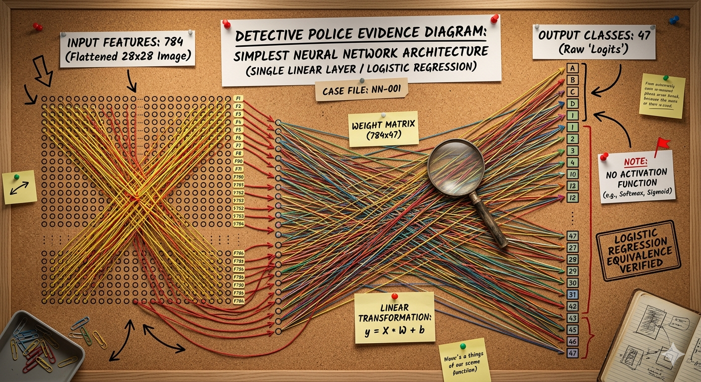
Build the simplest possible neural network — a single linear layer that maps 784 input features directly to 47 output classes. This is equivalent to logistic regression.

• Input: 784 features (28×28 flattened image)
• Output: 47 units (one per character class, no activation — raw "logits")

Evidence 3: The police diagram for their simple OCR network.

Steps:

1. Define a class inheriting from nn.Module
2. In __init__, call super().__init__() and create one nn.Linear(784, 47) layer
3. In forward(self, x), return the output of that layer
4. Create an instance and run a test forward pass to verify shapes

Useful functions:

• nn.Linear(in_features, out_features) — creates a fully connected layer with learnable weights and bias
• torch.argmax(tensor, dim=1) — returns the index of the maximum value along dimension 1 (the predicted class)
• sum(p.numel() for p in model.parameters()) — counts total learnable parameters

Task 02: Code (0.5 pts.)

class SimpleClassifier(nn.Module):
    def __init__(self):
        super().__init__()
        self.fc = nn.Linear(784, 47)

    # TODO: Finish the forward pass of the simple classifier
    def forward(self, x):
        pass

# TODO: Create an instance of your neural network
model = None

print(model)

total_params = sum(p.numel() for p in model.parameters())
print(f"\nTotal parameters: {total_params:,}")

test_batch = images_tensor[:4]           # (4, 784)

# TODO: Test forward pass on first 4 samples
output = None

print(f"\nInput shape:  {test_batch.shape}")
print(f"Output shape: {output.shape}")

# Get predicted classes (these are random since the model is untrained)
predictions = torch.argmax(output, dim=1)
print(f"Predicted classes: {predictions}")
print(f"(These are random - the model hasn't been trained yet!)")

SimpleClassifier(
  (fc): Linear(in_features=784, out_features=47, bias=True)
)

Total parameters: 36,895

Input shape:  torch.Size([4, 784])
Output shape: torch.Size([4, 47])
Predicted classes: tensor([ 1, 24,  1, 26])
(These are random - the model hasn't been trained yet!)

Task 02: Expected Output (0.5 pts.)

SimpleClassifier(
  (fc): Linear(in_features=784, out_features=47, bias=True)
)

Total parameters: 36,895

Input shape:  torch.Size([4, 784])
Output shape: torch.Size([4, 47])
Predicted classes: tensor([ 1, 24,  1, 26])
(These are random - the model hasn't been trained yet!)

Note: The output is 47 raw "logits" (one per class). The predicted class is the index of the largest logit (torch.argmax). Since the weights are random, the predictions are meaningless — but the shapes are correct!

Story Progression

"We've got a model," says Director Bryant, "but with thousands of images, you can't feed them all at once. You need to organize the data into batches." He's right — training on the full dataset at once would use too much memory. Instead, we split the data into small chunks and process one chunk at a time...

Task 03: Create a DataLoader (1 pt.)

Create a proper training pipeline from the full EMNIST dataset:

1. Create a TensorDataset from images_tensor and labels_tensor
2. Split into training (80%) and validation (20%) sets using random_split
3. Create DataLoaders for each — training with shuffle=True, validation with shuffle=False
4. Iterate over one training batch and print its shapes

Useful functions:

• TensorDataset(x_tensor, y_tensor) — wraps tensors into a dataset; indexing returns (x[i], y[i]) tuples
• random_split(dataset, [n_train, n_val]) — randomly splits a dataset into two non-overlapping parts
• DataLoader(dataset, batch_size=64, shuffle=True) — wraps a dataset to yield mini-batches; shuffle=True randomizes order each epoch

Task 03: Code (1 pt.)

from torch.utils.data import random_split

# TODO: Create TensorDataset from images and labels
full_dataset = None

print(f"Full dataset size: {len(full_dataset)}")

# TODO: Split into train (80%) and val (20%)
pass

train_dataset, val_dataset = random_split(full_dataset, [n_train, n_val])
print(f"Train: {len(train_dataset)}, Val: {len(val_dataset)}")

# TODO: Create DataLoaders with batch_size=64
train_loader = None
val_loader = None

# Print one batch to verify shapes
for batch_x, batch_y in train_loader:
    print(f"\nTraining batch: x={batch_x.shape}, y={batch_y.shape}")
    break

for batch_x, batch_y in val_loader:
    print(f"Validation batch: x={batch_x.shape}, y={batch_y.shape}")
    break

Full dataset size: 9400
Train: 7520, Val: 1880

Training batch: x=torch.Size([64, 784]), y=torch.Size([64])
Validation batch: x=torch.Size([64, 784]), y=torch.Size([64])

Task 03: Expected Output (1 pt.)

Full dataset size: 9400
Train: 7520, Val: 1880

Training batch: x=torch.Size([64, 784]), y=torch.Size([64])
Validation batch: x=torch.Size([64, 784]), y=torch.Size([64])

Note: Shuffling the training data each epoch prevents the model from memorizing the order of examples. We don't shuffle validation data because we just need a consistent accuracy measurement.

Story Progression

"Data's organized, model's defined," Director Bryant counts on his fingers. "Now we just need to... teach it?" That's training — the process of adjusting the model's weights by showing it examples and correcting its mistakes. The core of deep learning is a simple 3-step loop: compute the loss, compute the gradients, update the weights...

Evidence 4: The police's rough understanding of how training a network looks.

Task 04: Train the Single-Layer Model (0.5 pts.)

Train the SimpleClassifier on the training data and evaluate on the validation set.

Steps:

1. Create an Adam optimizer with lr=0.001 and a CrossEntropyLoss criterion
2. Train for 5 epochs, printing the average loss each epoch
3. After training, evaluate on the validation set and print accuracy

Useful functions:

• torch.optim.Adam(model.parameters(), lr=0.001) — creates an Adam optimizer that updates the model's weights
• nn.CrossEntropyLoss() — combines softmax + negative log-likelihood; takes raw logits and integer labels
• optimizer.zero_grad() — resets gradients to zero (PyTorch accumulates gradients by default!)
• loss.backward() — computes gradients of the loss w.r.t. all model parameters
• optimizer.step() — updates model parameters using the computed gradients
• torch.no_grad() — context manager that disables gradient computation (use during evaluation)

Task 04: Code (0.5 pts.)

simple_model = SimpleClassifier()

# TODO: Create optimizer and loss function
optimizer = None
criterion = None

for epoch in range(5):
    simple_model.train()
    total_loss = 0

    for batch_x, batch_y in train_loader:
        # TODO: For each batch: Forward pass, calculate loss, reset gradients, backprop, gradient descent
        logits = None       # forward pass
        loss = None    # compute loss

        optimizer.zero_grad()                # reset gradients

        pass                      # compute gradients
        pass                     # update weights

        total_loss += loss.item()

    avg_loss = total_loss / len(train_loader)
    print(f"Epoch {epoch+1}/5: avg loss = {avg_loss:.4f}")

# Evaluate on validation set
simple_model.eval()
correct = 0
total = 0

with torch.no_grad():
    for batch_x, batch_y in val_loader:
        logits = simple_model(batch_x)
        predictions = torch.argmax(logits, dim=1)
        correct += (predictions == batch_y).sum().item()
        total += batch_y.size(0)

simple_accuracy = correct / total
print(f"\nSimple model validation accuracy: {simple_accuracy:.4f} ({correct}/{total})")

Epoch 1/5: avg loss = 2.7509
Epoch 2/5: avg loss = 1.8086
Epoch 3/5: avg loss = 1.5426
Epoch 4/5: avg loss = 1.4084
Epoch 5/5: avg loss = 1.3297

Simple model validation accuracy: 0.6223 (1170/1880)

Task 04: Expected Output (0.5 pts.)

Epoch 1/5: avg loss = 2.7509
Epoch 2/5: avg loss = 1.8086
Epoch 3/5: avg loss = 1.5426
Epoch 4/5: avg loss = 1.4084
Epoch 5/5: avg loss = 1.3297

Simple model validation accuracy: 0.6223 (1170/1880)

The loss should decrease each epoch — this means the model is learning! The accuracy won't be amazing since this is just a single linear layer (equivalent to logistic regression), but it should be well above random chance (1/47 ≈ 2%). Take note of this accuracy — we'll try to beat it next.

Story Progression

The single-layer classifier is doing okay, but Detective Gaff isn't impressed. "The ransom note has some really messy handwriting. We need something more powerful." He's right — a single linear layer can only learn linear decision boundaries. To capture the complex patterns in handwritten characters, we need to go deeper...

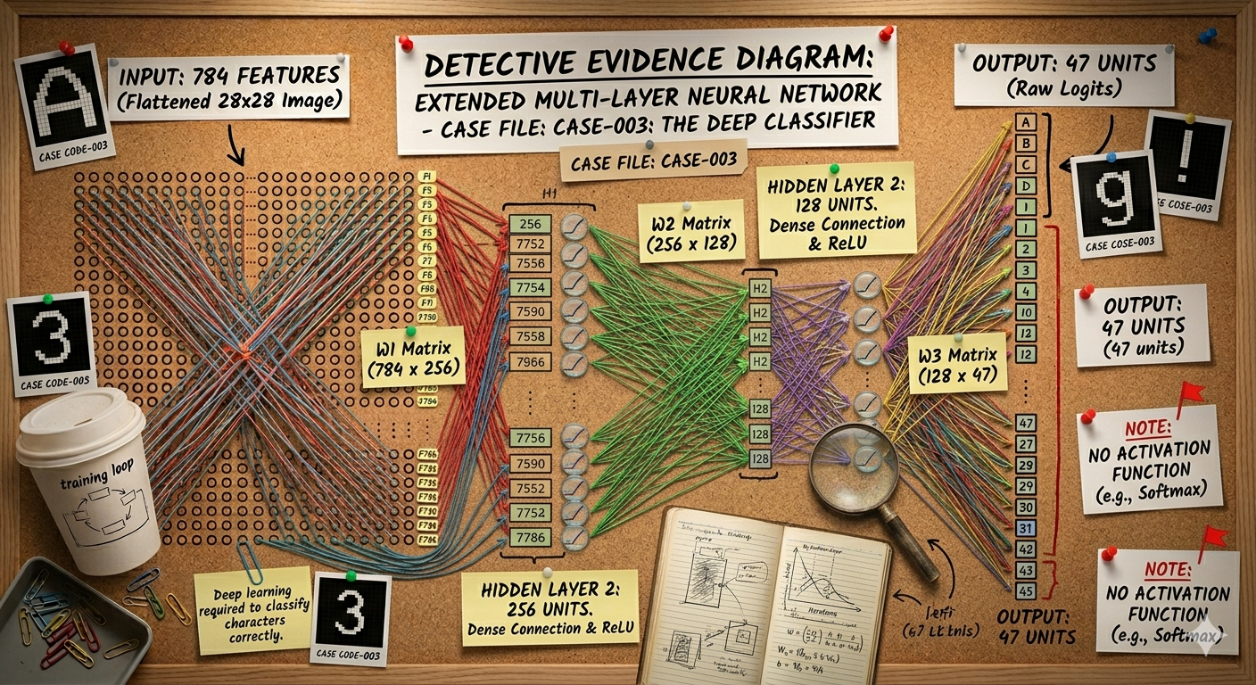
Task 05: Build a Multi-Layer FFN (1 pt.)

Extend the single-layer classifier into a proper feed-forward neural network with multiple layers and ReLU activations:

• Input: 784 features
• Hidden layer 1: 256 units + ReLU
• Hidden layer 2: 128 units + ReLU
• Output: 47 units (no activation — raw logits)

Evidence 5: The police's architecture for a deep neural network.

Steps:

1. Define a new nn.Module class with three nn.Linear layers
2. In forward(), pass the input through each layer, applying F.relu() after hidden layers
3. Create an instance and verify the shapes and parameter count

Useful functions:

• nn.Linear(in_features, out_features) — creates a fully connected layer
• F.relu(tensor) — applies ReLU activation (zeroes out negative values)
• Multiple layers are chained in forward(): x = F.relu(self.fc1(x)) then x = F.relu(self.fc2(x)) etc.

Task 05: Code (1 pt.)

# TODO: Finish the multi-layer FFN
class DeepClassifier(nn.Module):
    def __init__(self):
        super().__init__()
        pass

    def forward(self, x):
        pass

# TODO: Create an instance and print architecture
pass

total_params = sum(p.numel() for p in deep_model.parameters())
print(f"\nTotal parameters: {total_params:,}")

test_batch = images_tensor[:4]

# TODO: Test forward pass
pass

print(f"\nInput shape:  {test_batch.shape}")
print(f"Output shape: {output.shape}")

DeepClassifier(
  (fc1): Linear(in_features=784, out_features=256, bias=True)
  (fc2): Linear(in_features=256, out_features=128, bias=True)
  (fc3): Linear(in_features=128, out_features=47, bias=True)
)

Total parameters: 239,919

Input shape:  torch.Size([4, 784])
Output shape: torch.Size([4, 47])

Task 05: Expected Output (1 pt.)

DeepClassifier(
  (fc1): Linear(in_features=784, out_features=256, bias=True)
  (fc2): Linear(in_features=256, out_features=128, bias=True)
  (fc3): Linear(in_features=128, out_features=47, bias=True)
)

Total parameters: 239,919

Input shape:  torch.Size([4, 784])
Output shape: torch.Size([4, 47])

Note: The deep model has ~239K parameters vs ~37K for the simple model — about 6.5x more. The extra capacity comes from the hidden layers, which let the network learn non-linear features. The ReLU activations between layers are critical — without them, stacking linear layers would just collapse into a single linear transformation (as we discussed in lecture).

Story Progression

"Now that looks more like it," says Director Bryant, eyeing the 3-layer architecture. "More layers, more brainpower." But a bigger model doesn't mean a better model — it needs to be trained. Let's see if the extra depth actually helps...

Task 06: Train and Compare (1 pt.)

Train the DeepClassifier using the same setup as Task 04 (Adam optimizer, CrossEntropyLoss, 5 epochs), then compare its validation accuracy to the single-layer model.

Steps:

1. Train the deep model for 5 epochs (same loop as Task 04)
2. Evaluate on the validation set
3. Print both accuracies side by side
4. Answer the short-answer question below

Useful functions: Same as Task 04 — the training loop is identical, just with a different model!

Task 06: Code (1 pt.)

# TODO: Train the deep model (same pattern as Task 04)
pass

for epoch in range(5):
    pass

# Evaluate on validation set
deep_model.eval()
correct = 0
total = 0

with torch.no_grad():
    for batch_x, batch_y in val_loader:
        logits = deep_model(batch_x)
        predictions = torch.argmax(logits, dim=1)
        correct += (predictions == batch_y).sum().item()
        total += batch_y.size(0)

deep_accuracy = correct / total
print(f"\nDeep model validation accuracy: {deep_accuracy:.4f} ({correct}/{total})")

# Compare
print(f"\n{'='*50}")
print(f"Simple model (1 layer):  {simple_accuracy:.4f}")
print(f"Deep model   (3 layers): {deep_accuracy:.4f}")
print(f"Improvement: {(deep_accuracy - simple_accuracy)*100:+.1f} percentage points")

Epoch 1/5: avg loss = 2.6217
Epoch 2/5: avg loss = 1.4934
Epoch 3/5: avg loss = 1.2616
Epoch 4/5: avg loss = 1.0890
Epoch 5/5: avg loss = 0.9510

Deep model validation accuracy: 0.6686 (1257/1880)

==================================================
Simple model (1 layer):  0.6223
Deep model   (3 layers): 0.6686
Improvement: +4.6 percentage points

Task 06: Expected Output (0.5 pts.)

Epoch 1/5: avg loss = 2.6217
Epoch 2/5: avg loss = 1.4934
Epoch 3/5: avg loss = 1.2616
Epoch 4/5: avg loss = 1.0890
Epoch 5/5: avg loss = 0.9510

Deep model validation accuracy: 0.6686 (1257/1880)

==================================================
Simple model (1 layer):  0.6223
Deep model   (3 layers): 0.6686
Improvement: +4.6 percentage points

The deep model should achieve noticeably higher accuracy than the single-layer model. More layers + ReLU activations allow the network to learn non-linear decision boundaries.

Task 06: Short Answer (0.5 pts.)

Question: Why does the deep model outperform the single-layer model, even though both see the same data? What would happen if we removed the F.relu() calls between layers?

Answer: [ANSWER]

Story Progression

The multi-layer classifier is significantly better at reading the messy handwriting! You've now mastered the core PyTorch skills you'll need for Homework 04:

1. Tensors — creating them, converting from NumPy, choosing dtypes
2. nn.Module — defining model architectures with __init__ and forward
3. Dataset and DataLoader — organizing data into shuffled mini-batches
4. The training loop — zero_grad() → backward() → step(), plus torch.no_grad() evaluation
5. Multi-layer FFNs — stacking linear layers with ReLU activations

In HW04, you'll build this same architecture from scratch (implementing your own backpropagation!), then compare your version to PyTorch's built-in tools. Time to file your report!

Task 07: Generate Police Report (0 pts.)

Run the code cell below to generate a report for the Police and submit it on Canvas!

Task 07: Code (0 pts.)

import os, json

ASS_PATH = "nd-cse-30124-homeworks/labs"
ASS = "lab03"

try:
    from google.colab import _message, files

    repo_ipynb_path = f"/content/{ASS_PATH}/{ASS}/{ASS}.ipynb"

    nb = _message.blocking_request("get_ipynb", timeout_sec=1)["ipynb"]

    os.makedirs(os.path.dirname(repo_ipynb_path), exist_ok=True)
    with open(repo_ipynb_path, "w", encoding="utf-8") as f:
        json.dump(nb, f)

    !jupyter nbconvert --to html "{repo_ipynb_path}"
    files.download(repo_ipynb_path.replace(".ipynb", ".html"))
except:
    import subprocess

    nb_fp = os.getcwd() + f'/{ASS}.ipynb'
    print(os.getcwd())

    subprocess.run(["jupyter", "nbconvert", "--to", "html", nb_fp], check=True)
finally:
    print('[WARNING]: Unable to export notebook as .html')

[NbConvertApp] Converting notebook /content/nd-cse-30124-homeworks/labs/lab03/lab03.ipynb to html
[NbConvertApp] WARNING | Alternative text is missing on 1 image(s).
[NbConvertApp] Writing 355721 bytes to /content/nd-cse-30124-homeworks/labs/lab03/lab03.html

[WARNING]: Unable to export notebook as .html